Gaussian and exponential spatial covariance

Compare two covariance models with the same refractive index standard deviation and the same length parameter. Their definitions differ: Gaussian covariance is sigma_n**2 * exp(-r**2 / (2 * ell**2)), while exponential covariance is sigma_n**2 * exp(-r / ell). Equal parameters therefore do not give identical real-space profiles or scattering spectra. Here, r is the distance between two points in the medium. The covariance describes how their refractive-index fluctuations vary together as that distance increases.

Both random-volume generators use Gaussian probability distributions; the covariance choice describes spatial correlations. The phase functions below come from numerical first-order finite-sample ensembles and are normalized per steradian, not per degree.

from bornsim.medium.random_medium import GaussianMedium, ExponentialMedium

import matplotlib.pyplot as plt
import numpy as np

from bornsim import AngularSampling, EnsembleSampling, Grid, Solver, Source
from bornsim.units import ureg

correlation_length = 120 * ureg.nanometer

distance_between_points = np.linspace(0, 500, 301) * ureg.nanometer

source_configuration_1 = Source(wavelength=633 * ureg.nanometer)

solver = Solver(
    source=source_configuration_1,
    order=1,
)

sampling = AngularSampling(
    start=0 * ureg.degree,
    end=180 * ureg.degree,
    n_points=181,
)

grid = Grid(
    shape=(6, 6, 6),
    spacing=40 * ureg.nanometer,
)

ensemble_sampling = EnsembleSampling(
    realizations=8,
    seed=42,
)

preview_volumes = {}

Compare numerical scattering

figure, (covariance_axis, phase_axis) = plt.subplots(1, 2, figsize=(11, 4), layout="constrained")

for correlation, color in (("gaussian", "C0"), ("exponential", "C1")):
    medium_type = {
        "gaussian": GaussianMedium,
        "exponential": ExponentialMedium,
    }[correlation]

    medium = medium_type(
        refractive_index_std=0.01,
        correlation_length=correlation_length,
        background_refractive_index=1.33,
    )

    # Show the first ensemble realization on the same grid used for scattering.
    preview_volume = medium.to_volume(
        grid=grid,
        seed=ensemble_sampling.seeds[0],
    )

    preview_volumes[correlation] = preview_volume

    distance_over_correlation_length = (distance_between_points / correlation_length).to("dimensionless").magnitude

    normalized_covariance = (
        np.exp(-(distance_over_correlation_length**2) / 2)
        if correlation == "gaussian"
        else np.exp(-distance_over_correlation_length)
    )

    result = solver.ensemble(
        medium=medium,
        grid=grid,
        ensemble_sampling=ensemble_sampling,
        sampling=sampling,
    )

    averaged = result.azimuth_average()

    covariance_axis.plot(
        distance_between_points.magnitude,
        normalized_covariance,
        color=color,
        label=correlation.capitalize(),
    )

    phase_axis.semilogy(
        result.angles.to("degree").magnitude,
        averaged.phase_function.to("1 / steradian").magnitude[0],
        color=color,
        label=f"{correlation.capitalize()}, g = {result.g.magnitude[0]:.3f}",
    )

    print(f"{correlation}: μs = {result.mu_s[0].to('1 / millimeter')}")

covariance_axis.set(xlabel="Distance between points r (nm)", ylabel="Cn(r) / σn²", title="Spatial covariance")

phase_axis.set(xlabel="Scattering angle (degrees)", ylabel="Phase function p (sr⁻¹)", title="Directional scattering")

for axis in (covariance_axis, phase_axis):
    axis.grid(alpha=0.25)

    axis.legend(frameon=False)

figure.suptitle("Same ℓ = 120 nm and σn = 0.01; different covariance models")

plt.show()

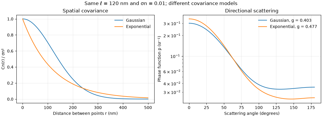
gaussian: μs = 1.0545345044304941 / millimeter
exponential: μs = 0.9101819512925958 / millimeter

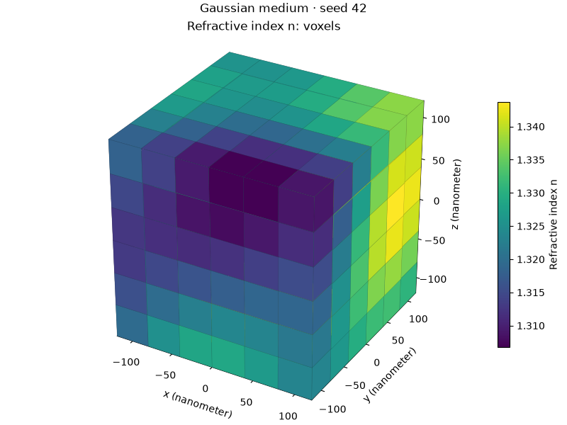
Gaussian medium in 3D

Show one finite input sample with its physical spatial axes.

preview_volume = preview_volumes["gaussian"]

medium_figure = preview_volume.plot_3d(
    backend="matplotlib",
    mode="voxels",
    field="refractive_index",
)

medium_figure.suptitle(f"Gaussian medium · seed {ensemble_sampling.seeds[0]}")

plt.show()

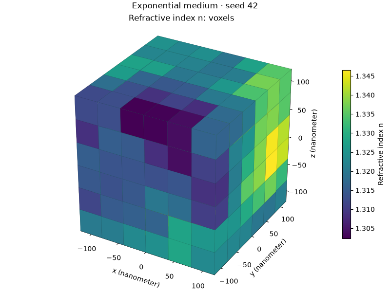
Exponential medium in 3D

Show one finite input sample with its physical spatial axes.

preview_volume = preview_volumes["exponential"]

medium_figure = preview_volume.plot_3d(
    backend="matplotlib",
    mode="voxels",
    field="refractive_index",
)

medium_figure.suptitle(f"Exponential medium · seed {ensemble_sampling.seeds[0]}")

plt.show()