Normalized phase function

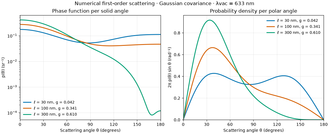
Compare finite-sample ensemble phase functions for three Gaussian covariance lengths at a vacuum wavelength of 633 nm. The phase function is a probability density per steradian, normalized over solid angle. The corresponding polar-angle density includes the factor 2*pi*sin(theta) and integrates over radians.

The medium is three-dimensional. The displayed curves explicitly average the sampled azimuthal directions; individual finite samples need not have rotational symmetry.

from bornsim.medium.random_medium import GaussianMedium

import matplotlib.pyplot as plt
import numpy as np

from bornsim import AngularSampling, EnsembleSampling, Grid, Solver, Source
from bornsim.units import ureg

Compare correlation lengths

Longer covariance lengths can produce more forward-peaked scattering. The same result provides the phase function and its mean cosine, g.

source_configuration_1 = Source(wavelength=633 * ureg.nanometer)

solver = Solver(
    source=source_configuration_1,
    order=1,
)

sampling = AngularSampling(
    start=0 * ureg.degree,
    end=180 * ureg.degree,
    n_points=181,
)

grid = Grid(
    shape=(6, 6, 6),
    spacing=40 * ureg.nanometer,
)

ensemble_sampling = EnsembleSampling(
    realizations=8,
    seed=42,
)

preview_volumes = {}

Compare numerical scattering

figure, (phase_axis, density_axis) = plt.subplots(1, 2, figsize=(11, 4.5), layout="constrained")

for length_nm, color in zip((30, 100, 300), ("#0072B2", "#D55E00", "#009E73")):
    medium = GaussianMedium(
        correlation_length=length_nm * ureg.nanometer,
        background_refractive_index=1.33,
        refractive_index_std=0.01,
    )

    # Show the first ensemble realization on the same grid used for scattering.
    preview_volume = medium.to_volume(
        grid=grid,
        seed=ensemble_sampling.seeds[0],
    )

    preview_volumes[length_nm] = preview_volume

    result = solver.ensemble(
        medium=medium,
        grid=grid,
        ensemble_sampling=ensemble_sampling,
        sampling=sampling,
    )

    averaged = result.azimuth_average()

    phase = averaged.phase_function.magnitude[0]

    theta = result.angles.to("radian").magnitude

    polar_density = 2 * np.pi * phase * np.sin(theta)

    label = f"ℓ = {length_nm} nm, g = {result.g.magnitude[0]:.3f}"

    phase_axis.semilogy(result.angles.to("degree").magnitude, phase, color=color, label=label, linewidth=2)

    density_axis.plot(
        result.angles.to("degree").magnitude,
        polar_density,
        color=color,
        label=label,
        linewidth=2,
    )

phase_axis.set(title="Phase function per solid angle", ylabel="p(θ) (sr⁻¹)")

density_axis.set(title="Probability density per polar angle", ylabel="2π p(θ) sin θ (rad⁻¹)", ylim=(0, None))

for axis in (phase_axis, density_axis):
    axis.set(xlabel="Scattering angle θ (degrees)", xlim=(0, 180), xticks=np.arange(0, 181, 30))

    axis.grid(alpha=0.25)

    axis.legend(frameon=False, fontsize=9)

figure.suptitle("Numerical first-order scattering · Gaussian covariance · λvac = 633 nm")

plt.show()

30 nm correlation length in 3D

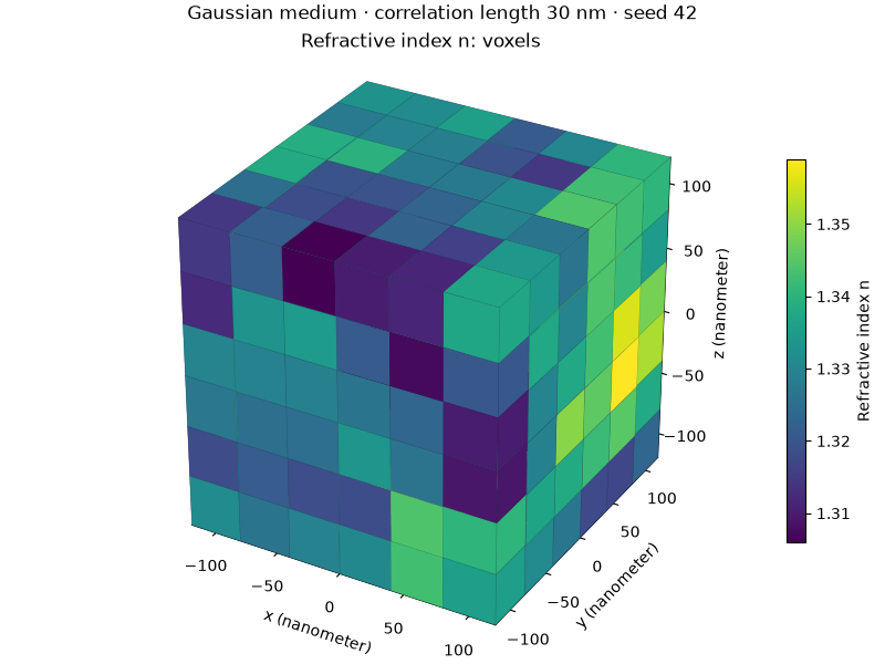
Show one finite input sample with its physical spatial axes.

preview_volume = preview_volumes[30]

medium_figure = preview_volume.plot_3d(
    backend="matplotlib",
    mode="voxels",
    field="refractive_index",
)

medium_figure.suptitle(f"Gaussian medium · correlation length 30 nm · seed {ensemble_sampling.seeds[0]}")

plt.show()

100 nm correlation length in 3D

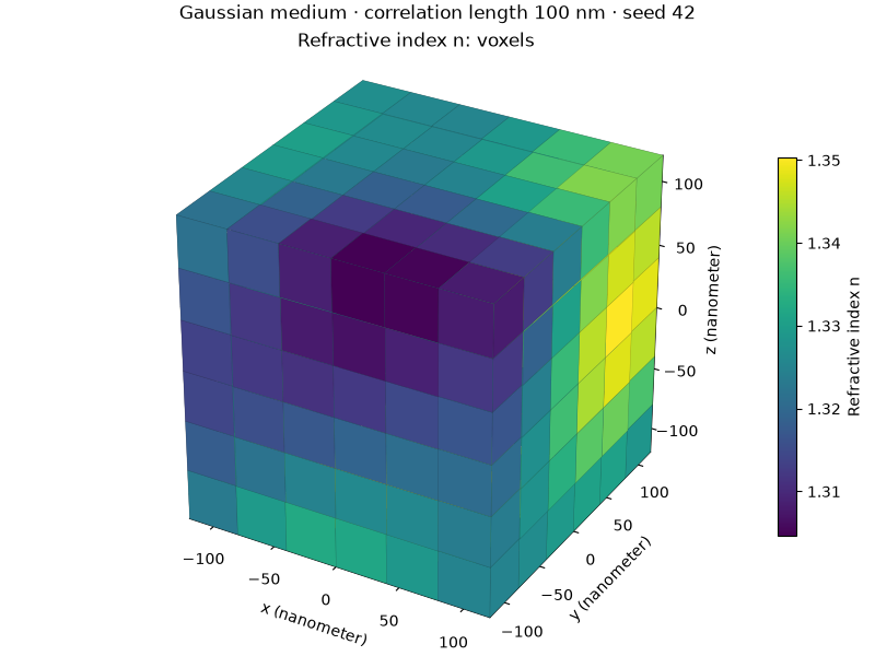
Show one finite input sample with its physical spatial axes.

preview_volume = preview_volumes[100]

medium_figure = preview_volume.plot_3d(
    backend="matplotlib",
    mode="voxels",
    field="refractive_index",
)

medium_figure.suptitle(f"Gaussian medium · correlation length 100 nm · seed {ensemble_sampling.seeds[0]}")

plt.show()

300 nm correlation length in 3D

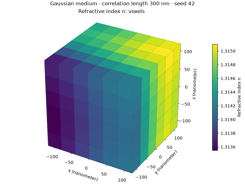
Show one finite input sample with its physical spatial axes.

preview_volume = preview_volumes[300]

medium_figure = preview_volume.plot_3d(
    backend="matplotlib",
    mode="voxels",
    field="refractive_index",
)

medium_figure.suptitle(f"Gaussian medium · correlation length 300 nm · seed {ensemble_sampling.seeds[0]}")

plt.show()