Visualize seeded three-dimensional random media

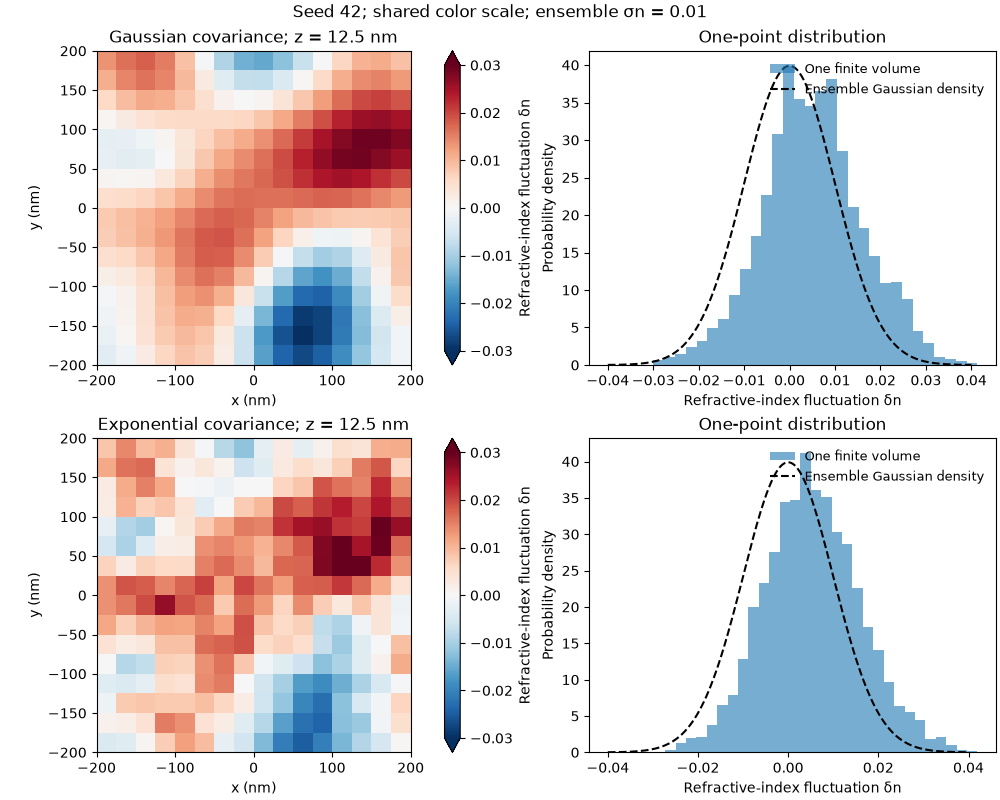
Explore the full three-dimensional sample for each spatial covariance model. Drag to rotate, scroll to zoom, and hover to inspect the refractive index. Regions with lower refractive index are transparent; regions with higher refractive index are more opaque. Opacity is a display setting, not absorption. Histograms and central slices follow as secondary checks of the same seeded fields.

Both models have Gaussian one-point probability distributions. Correlated voxels in one finite sample are not independent observations, so a voxel histogram need not match the ensemble Gaussian density closely. BornSim does not recenter or rescale each realization to impose its mean or variance. Finite voxel resolution and the cropped synthesis box also affect statistics.

from bornsim.medium.random_medium import GaussianMedium, ExponentialMedium

import sys

import matplotlib.pyplot as plt
import numpy as np

from bornsim import Grid
from bornsim.units import ureg

grid_shape = (16, 16, 16)

voxel_spacing = 25 * ureg.nanometer

grid = Grid(
    shape=grid_shape,
    spacing=voxel_spacing,
)

refractive_index_std = 0.01

half_sample_width_nm = grid_shape[0] * voxel_spacing.to("nanometer").magnitude / 2

slice_extent_nm = (-half_sample_width_nm, half_sample_width_nm, -half_sample_width_nm, half_sample_width_nm)

# Evaluate the ensemble probability density at these refractive-index fluctuations.
refractive_index_fluctuations = np.linspace(-4 * refractive_index_std, 4 * refractive_index_std, 301)

gaussian_probability_density = np.exp(-(refractive_index_fluctuations**2) / (2 * refractive_index_std**2)) / (
    np.sqrt(2 * np.pi) * refractive_index_std
)

volumes_by_covariance = {}

for covariance_model in ("gaussian", "exponential"):
    medium_type = {
        "gaussian": GaussianMedium,
        "exponential": ExponentialMedium,
    }[covariance_model]

    random_medium = medium_type(
        refractive_index_std=refractive_index_std,
        correlation_length=75 * ureg.nanometer,
        background_refractive_index=1.33,
    )

    sampled_volume = random_medium.to_volume(
        grid=grid,
        seed=42,
    )

    volumes_by_covariance[covariance_model] = sampled_volume

    print(
        f"{covariance_model}: sample mean = {sampled_volume.delta_refractive_index.mean():.4g}, sample std = {sampled_volume.delta_refractive_index.std():.4g}"
    )

gaussian: sample mean = 0.005049, sample std = 0.01101
exponential: sample mean = 0.005348, sample std = 0.01069

Gaussian volume with increasing opacity

View the full Gaussian sample first. The opacity ramp uses this sample’s refractive index range; equal opacity across different samples need not mean equal refractive index. Pass --no-browser to run without opening tabs, as the docs builder does.

gaussian_volume = volumes_by_covariance["gaussian"]

gaussian_figure = gaussian_volume.plot_3d(
    field="refractive_index",
    surface_count=16,
    opacity=0.2,
    opacity_scale="increasing",
)

if "--no-browser" not in sys.argv:
    gaussian_figure.show(renderer="browser")

Exponential volume with increasing opacity

Compare the exponential sample in its own interactive view with the same rendering settings. Correlation length conventions differ between models.

exponential_volume = volumes_by_covariance["exponential"]

exponential_figure = exponential_volume.plot_3d(
    field="refractive_index",
    surface_count=16,
    opacity=0.2,
    opacity_scale="increasing",
)

if "--no-browser" not in sys.argv:
    exponential_figure.show(renderer="browser")

Secondary checks: central slices and one-point distributions

Slices show one sampled plane, while histograms describe the finite field’s one-point distribution. Neither replaces the complete spatial volume above.

slice_figure, slice_and_histogram_axes = plt.subplots(2, 2, figsize=(10, 8), layout="constrained")

for covariance_row, covariance_model in enumerate(("gaussian", "exponential")):
    sampled_volume = volumes_by_covariance[covariance_model]

    slice_axis, histogram_axis = slice_and_histogram_axes[covariance_row]

    slice_image = slice_axis.imshow(
        sampled_volume.delta_refractive_index[:, :, grid_shape[2] // 2].T,
        origin="lower",
        extent=slice_extent_nm,
        cmap="RdBu_r",
        vmin=-3 * refractive_index_std,
        vmax=3 * refractive_index_std,
    )

    slice_z_nm = sampled_volume.positions[0, 0, grid_shape[2] // 2, 2].to("nanometer").magnitude

    slice_axis.set(
        xlabel="x (nm)", ylabel="y (nm)", title=f"{covariance_model.capitalize()} covariance; z = {slice_z_nm:g} nm"
    )

    slice_figure.colorbar(slice_image, ax=slice_axis, label="Refractive-index fluctuation δn", extend="both")

    histogram_axis.hist(
        sampled_volume.delta_refractive_index.ravel(), bins=30, density=True, alpha=0.6, label="One finite volume"
    )

    histogram_axis.plot(
        refractive_index_fluctuations,
        gaussian_probability_density,
        "k--",
        label="Ensemble Gaussian density",
    )

    histogram_axis.set(
        xlabel="Refractive-index fluctuation δn", ylabel="Probability density", title="One-point distribution"
    )

    histogram_axis.legend(frameon=False, loc="upper right", fontsize=9)

slice_figure.suptitle("Seed 42; shared color scale; ensemble σn = 0.01")

plt.show()