Wavelength dependence of scattering and anisotropy

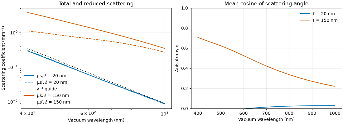
Sweep vacuum wavelength at fixed background refractive index, refractive-index fluctuation strength, and Gaussian covariance length. Total scattering and reduced scattering are different observables: forward scattering increases anisotropy and reduces the contribution to mu_s_prime = mu_s * (1 - g).

These are numerical first-order finite-sample coefficients. The background refractive index and fluctuation statistics are held constant, so material dispersion is not included. The wavelength-to-the-minus-four guide applies in the short-correlation limit, not generally at every covariance length.

from bornsim.medium.random_medium import GaussianMedium

import matplotlib.pyplot as plt
import numpy as np

from bornsim import AngularSampling, EnsembleSampling, Grid, Solver, Source
from bornsim.units import ureg

wavelengths = np.linspace(400, 1000, 13) * ureg.nanometer

grid = Grid(
    shape=(6, 6, 6),
    spacing=40 * ureg.nanometer,
)

ensemble_sampling = EnsembleSampling(
    realizations=8,
    seed=42,
)

preview_volumes = {}

Compare numerical scattering

figure, (coefficient_axis, anisotropy_axis) = plt.subplots(1, 2, figsize=(11, 4), layout="constrained")

for length_nm, color in ((20, "#0072B2"), (150, "#D55E00")):
    medium = GaussianMedium(
        refractive_index_std=0.01,
        correlation_length=length_nm * ureg.nanometer,
        background_refractive_index=1.33,
    )

    # Show the first ensemble realization on the same grid used for scattering.
    preview_volume = medium.to_volume(
        grid=grid,
        seed=ensemble_sampling.seeds[0],
    )

    preview_volumes[length_nm] = preview_volume

    coefficients = []

    reduced = []

    anisotropy = []

    for wavelength in wavelengths:
        source_configuration_1 = Source(wavelength=wavelength)

        sampling_configuration_1 = AngularSampling(angles=[0] * ureg.radian)

        solver = Solver(
            source=source_configuration_1,
            order=1,
            sampling=sampling_configuration_1,
        )

        result = solver.ensemble(
            medium=medium,
            grid=grid,
            ensemble_sampling=ensemble_sampling,
        )

        coefficients.append(result.mu_s.to("1 / millimeter").magnitude[0])

        reduced.append(result.mu_s_prime.to("1 / millimeter").magnitude[0])

        anisotropy.append(result.g.magnitude[0])

    label = f"ℓ = {length_nm} nm"

    coefficient_axis.loglog(wavelengths.magnitude, coefficients, color=color, label=f"μs, {label}")

    coefficient_axis.loglog(wavelengths.magnitude, reduced, "--", color=color, label=f"μs′, {label}")

    anisotropy_axis.plot(
        wavelengths.magnitude,
        anisotropy,
        color=color,
        label=label,
    )

    if length_nm == 20:
        guide = coefficients[-1] * (wavelengths.magnitude[-1] / wavelengths.magnitude) ** 4

        coefficient_axis.loglog(wavelengths.magnitude, guide, ":", color="black", label="λ⁻⁴ guide")

coefficient_axis.set(ylabel="Scattering coefficient (mm⁻¹)", title="Total and reduced scattering")

anisotropy_axis.set(ylabel="Anisotropy g", title="Mean cosine of scattering angle", ylim=(0, 1))

for axis in (coefficient_axis, anisotropy_axis):
    axis.set(xlabel="Vacuum wavelength (nm)")

    axis.legend(frameon=False)

    axis.grid(alpha=0.25)

plt.show()

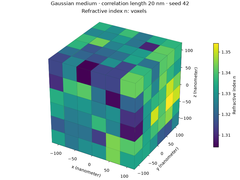
20 nm correlation length in 3D

Show one finite input sample with its physical spatial axes.

preview_volume = preview_volumes[20]

medium_figure = preview_volume.plot_3d(
    backend="matplotlib",
    mode="voxels",
    field="refractive_index",
)

medium_figure.suptitle(f"Gaussian medium · correlation length 20 nm · seed {ensemble_sampling.seeds[0]}")

plt.show()

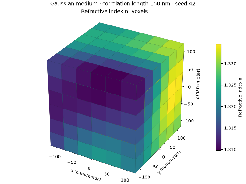
150 nm correlation length in 3D

Show one finite input sample with its physical spatial axes.

preview_volume = preview_volumes[150]

medium_figure = preview_volume.plot_3d(
    backend="matplotlib",
    mode="voxels",
    field="refractive_index",
)

medium_figure.suptitle(f"Gaussian medium · correlation length 150 nm · seed {ensemble_sampling.seeds[0]}")

plt.show()