Result plots and interactive 3D views

Use plotting methods directly on a result, then call plt.show() to display angular Matplotlib figures. The docs embed interactive Plotly volumes and phase surfaces; drag to rotate and scroll to zoom.

The phase surface represents directions on a sphere. Its radius and color are probability densities in inverse steradians, not spatial coordinates. The ensemble angular curves show a sampled meridian about incident +z. Use result.azimuth_average() to request an averaged curve explicitly. The 3D surface retains each azimuth direction, showing directional structure in the ensemble intensity average.

from bornsim.medium.random_medium import GaussianMedium

import sys

import matplotlib.pyplot as plt

from bornsim import EnsembleSampling, Grid, Solver, Source
from bornsim.units import ureg

grid = Grid(
    shape=(4, 4, 4),
    spacing=50 * ureg.nanometer,
)

medium = GaussianMedium(
    correlation_length=100 * ureg.nanometer,
    background_refractive_index=1.33,
    refractive_index_std=0.01,
)

source_configuration_1 = Source(wavelength=633 * ureg.nanometer)

solver = Solver(
    source=source_configuration_1,
    order=3,
)

ensemble_sampling_configuration_1 = EnsembleSampling(
    realizations=4,
    seed=42,
)

result = solver.ensemble(
    medium=medium,
    grid=grid,
    ensemble_sampling=ensemble_sampling_configuration_1,
)

Differential scattering

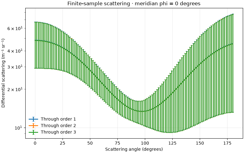
Differential scattering retains its physical units of inverse metres per steradian. Ensemble results also show standard errors on this plot.

result.plot(log_y=True)

plt.show()

Normalized phase function

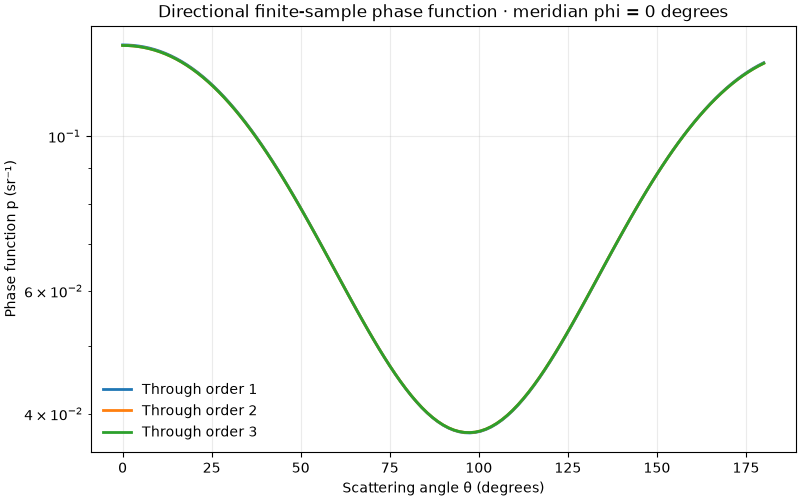
Dividing by the integrated coefficient gives a density per steradian. The normalization is over solid angle, including the sin(theta) measure.

result.plot_phase_function(log_y=True)

plt.show()

Polar meridian cut

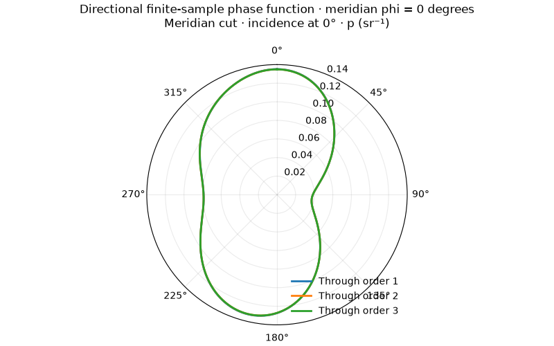
The incident beam points towards 0 degrees, at the top of the plot.

result.plot_phase_function(view="polar")

plt.show()

Three-dimensional directional surface

Plot the sampled polar and azimuth directions without azimuth averaging. Here four realizations contribute to the ensemble intensity average.

phase_figure = result.plot_phase_function(view="3d")

if "--no-browser" not in sys.argv:
    phase_figure.show(renderer="browser")

Numerical field terms

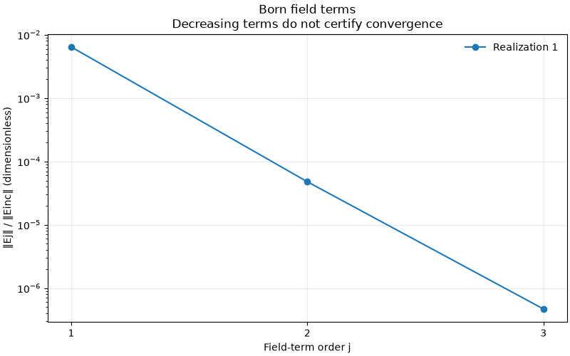
A fixed random volume need not be axisymmetric. Its field norms can be inspected without inferring a normalized phase function from one cut. Decreasing terms do not certify Born convergence.

volume = medium.to_volume(
    grid=grid,
    seed=42,
)

numerical = solver.solve(target=volume)

numerical.plot_field_norms()

plt.show()

Inspect the medium in 3D

Inspect the actual finite input sample with physical spatial axes. Drag to rotate and scroll to zoom in the embedded browser view. Regions with higher refractive index are more opaque; opacity is not absorption.

medium_figure = volume.plot_3d(
    mode="volume",
    field="refractive_index",
    opacity_scale="increasing",
)

if "--no-browser" not in sys.argv:
    medium_figure.show(renderer="browser")