Save results and inspect calculation provenance

Save a numerical result and restore it with its physical units, complex amplitudes, diagnostics, and original calculation settings. The versioned NumPy archive uses JSON metadata and loads without pickle.

This example uses a temporary directory so running the gallery leaves no data files behind. For a persistent archive, pass your desired filename to result.save(path="scattering.npz"). Archives contain results rather than the original input voxel field. Retain manually supplied fields separately; generated-volume provenance records the medium and seed, with a field hash to identify the exact input. Exact regeneration depends on software versions.

from bornsim.medium.random_medium import GaussianMedium

from pathlib import Path
from tempfile import TemporaryDirectory

import sys

import matplotlib.pyplot as plt
import numpy as np

from bornsim import Grid, Result, Solver, Source
from bornsim.units import ureg

grid = Grid(
    shape=(4, 4, 4),
    spacing=40 * ureg.nanometer,
)

medium = GaussianMedium(
    correlation_length=80 * ureg.nanometer,
    background_refractive_index=1.33,
    refractive_index_std=0.01,
)

volume = medium.to_volume(
    grid=grid,
    seed=42,
)

source_configuration_1 = Source(wavelength=633 * ureg.nanometer)

solver = Solver(
    source=source_configuration_1,
    order=3,
)

result = solver.solve(target=volume)

with TemporaryDirectory() as directory:
    path = result.save(path=Path(directory) / "scattering.npz")

    restored = Result.load(path=path)

Inspect settings and retained amplitudes

The arrays have been copied from the archive; they remain usable after the temporary directory is removed. Loading preserves the recorded versions.

print(f"BornSim version: {restored.provenance['bornsim_version']}")

print(f"NumPy version: {restored.provenance['numpy_version']}")

print(f"Seed: {restored.provenance['seed']}")

print(f"Grid: {restored.provenance['grid']}")

print(f"Medium: {restored.provenance['medium']}")

print(f"Coefficient scope: {restored.provenance['coefficient_scope']}")

print(f"Wavelength: {restored.source.wavelength.to('nanometer')}")

print(f"Complex amplitudes retained: {np.iscomplexobj(restored.amplitudes.magnitude)}")

BornSim version: 0.5.1
NumPy version: 2.4.6
Seed: 42
Grid: {'shape': [4, 4, 4], 'spacing_m': 4e-08, 'background_refractive_index': 1.33, 'delta_refractive_index_sha256': 'af423859f3fc7019d700fa3e969b1a81b72e4f170e654b08fae09eea22681b04'}
Medium: {'background_refractive_index': 1.33, 'refractive_index_std': 0.01, 'correlation_length_m': 8e-08, 'correlation': 'gaussian', 'smoothness': None}
Coefficient scope: finite-sample
Wavelength: 632.9999999999999 nanometer
Complex amplitudes retained: True

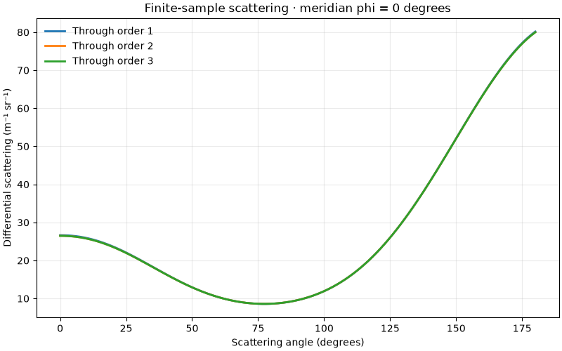
Plot restored scattering

Full angular sampling supplies normalized phase functions and finite-sample coefficients. They are not infinite-medium material transport coefficients.

restored.plot()

plt.show()

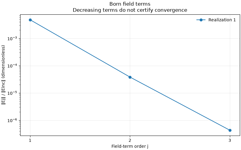
Plot restored field diagnostics

Decreasing field terms do not certify Born convergence.

restored.plot_field_norms()

plt.show()

Inspect the medium in 3D

Inspect the actual finite input sample with physical spatial axes. Drag to rotate and scroll to zoom in the embedded browser view. Regions with higher refractive index are more opaque; opacity is not absorption.

medium_figure = volume.plot_3d(
    mode="volume",
    field="refractive_index",
    opacity_scale="increasing",
)

if "--no-browser" not in sys.argv:
    medium_figure.show(renderer="browser")