Distribution Classes#

The Distribution classes define the methods for generating particle sizes used in the simulation. These classes provide flexibility in modeling particles of varying sizes according to different statistical distributions, such as normal, log-normal, Weibull, and more. This allows for realistic simulation of particle populations with varying size characteristics.

Available Distribution Classes#

The following are the available particle size distribution classes in FlowCyPy:
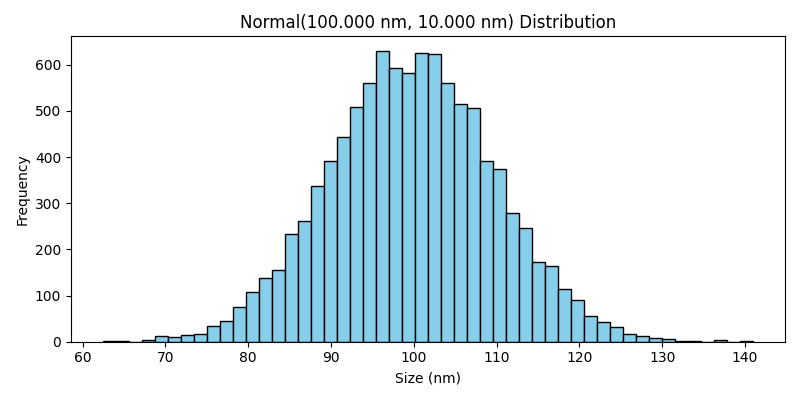
Normal Distribution#

The Normal class generates particle sizes that follow a normal (Gaussian) distribution. This distribution is characterized by a symmetric bell curve, where most particles are concentrated around the mean size, with fewer particles at the extremes.

../_images/Normal.png
class Normal(mean, standard_deviation, cutoff=None)[source]#

Bases: Base

Normal (Gaussian) distribution with optional hard cutoff.

This class represents a normal distribution for a particle property such as diameter or refractive index. It supports an optional hard lower cutoff that turns the sampler into a truncated normal distribution conditional on

\[X \ge x_{\mathrm{cut}}.\]

Without cutoff#

Samples are drawn from:

\[X \sim \mathcal{N}(\mu, \sigma^2).\]

With cutoff#

Samples are drawn from the conditional distribution:

\[X \mid X \ge x_{\mathrm{cut}}.\]

This is implemented by inverse CDF sampling on the restricted probability interval [F(x_cut), 1) where F is the Gaussian CDF. This avoids rejection sampling and provides predictable performance even when the cutoff is far into the tail.

param mean:

Mean value \(\mu\) of the distribution, with units.

type mean:

TypedUnit.units.AnyUnit

param standard_deviation:

Standard deviation \(\sigma\) of the distribution, with the same units as mean.

type standard_deviation:

TypedUnit.units.AnyUnit

param cutoff:

Optional hard minimum value. If provided, generated samples satisfy x >= cutoff by construction.

type cutoff:

TypedUnit.units.AnyUnit | None

apply_cutoff(cutoff, reduce_concentration_consistently=True)[source]#

Return a truncated Normal distribution and an optional concentration multiplier.

Interpretation#

  • The returned distribution samples from X | X >= cutoff.

  • If reduce_concentration_consistently is True, the returned multiplier is P(X >= cutoff) so that concentration can be scaled consistently with the same underlying distribution.

  • If False, the multiplier is 1.0.

param cutoff:

Hard minimum value for truncation.

param reduce_concentration_consistently:

Whether to return the survival fraction as a concentration multiplier.

returns:

truncated_distribution is a new instance with cutoff set. concentration_multiplier is either the survival fraction or 1.0.

rtype:

truncated_distribution, concentration_multiplier

Parameters:
  • cutoff (AnyUnit)

  • reduce_concentration_consistently (bool)

Return type:

Tuple[Normal, float]

cdf(x)[source]#

Evaluate the Gaussian CDF at x (ignoring any cutoff).

Parameters:

x (AnyUnit) – Quantity with the same units as mean.

Returns:

CDF value in [0, 1].

Return type:

float

cutoff: AnyUnit | None = None#
generate(n_samples)#

Generate a distribution of scatterer diameters.

Parameters:

n_samples (AnyUnit)

get_pdf(x=None, x_min=-3, x_max=3, n_samples=200)[source]#

Return x values and the PDF.

If cutoff is None, this returns the standard normal PDF.

If cutoff is set, this returns the truncated PDF:

pdf_trunc(x) = pdf(x) / P(X >= cutoff) for x >= cutoff

0 otherwise

Parameters:
  • x (ndarray) – Optional x grid with units. If not provided, a default grid is generated.

  • x_min (float) – Lower bound in sigma units for the default grid.

  • x_max (float) – Upper bound in sigma units for the default grid.

  • n_samples (int) – Number of points used for the default grid.

Returns:

x with units and pdf as a unitless NumPy array.

Return type:

Tuple[np.ndarray, np.ndarray]

mean: AnyUnit#
standard_deviation: AnyUnit#
survival_fraction_above(cutoff)[source]#

Compute the survival fraction above a cutoff, P(X >= cutoff).

This quantity is the concentration multiplier you would apply if you interpret the cutoff as physically removing all values below cutoff from an otherwise unchanged population.

Parameters:

cutoff (AnyUnit) – Hard minimum value with the same units as mean.

Returns:

Survival fraction in [0, 1].

Return type:

float

Parameters:
  • mean (AnyUnit)

  • standard_deviation (AnyUnit)

  • cutoff (AnyUnit | None)

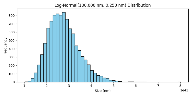
LogNormal Distribution#

The LogNormal class generates particle sizes based on a log-normal distribution. In this case, the logarithm of the particle sizes follows a normal distribution. This type of distribution is often used to model phenomena where the particle sizes are positively skewed, with a long tail towards larger sizes.

../_images/LogNormal.png
class LogNormal(mean, standard_deviation, cutoff=None)[source]#

Bases: Base

Log normal distribution with optional hard cutoff.

This class represents a log normal distribution for a positive particle property such as diameter or intensity. It supports an optional hard lower cutoff that turns the sampler into a truncated log normal distribution conditional on

\[X \ge x_{\mathrm{cut}}.\]

Definition#

A log normal random variable is defined by

\[\ln(X) \sim \mathcal{N}(\mu, \sigma^2),\]

which implies the density

\[f(x) = \frac{1}{x \sigma \sqrt{2\pi}} \exp\!\left(-\frac{(\ln x - \mu)^2}{2\sigma^2}\right), \quad x > 0.\]

Parameterization used here#

This implementation follows the NumPy and SciPy convention:

  • mean corresponds to \(\mu\), the mean of the underlying normal distribution of ln(X).

  • standard_deviation corresponds to \(\sigma\), the standard deviation of the underlying normal distribution of ln(X).

In other words, mean and standard_deviation are parameters in log space. If you want to specify the arithmetic mean and standard deviation in linear space, you must convert them to \(\mu\) and \(\sigma\) before creating this distribution.

Hard cutoff and truncation#

When cutoff is provided, sampling is performed from the conditional law X | X >= cutoff by inverse CDF sampling on the restricted probability interval [F(cutoff), 1) where F is the log normal CDF.

This provides an efficient way to emulate an idealized selection that removes all values below the cutoff. If you interpret the cutoff as a physical removal, you can compute the matching concentration multiplier via survival_fraction_above().

param mean:

Log space mean \(\mu\) with units carried for consistency with the rest of the framework. In practice, this should be dimensionless.

type mean:

TypedUnit.units.AnyUnit

param standard_deviation:

Log space standard deviation \(\sigma\). In practice, this should be dimensionless and strictly positive.

type standard_deviation:

TypedUnit.units.AnyUnit

param cutoff:

Optional hard minimum value for X in linear space, with the same units as the sampled property. If provided, generated samples satisfy x >= cutoff by construction.

type cutoff:

TypedUnit.units.AnyUnit | None

Notes

  • The sampled values are always positive by definition.

  • If you use this distribution for diameter, the log space parameters should be calibrated carefully, because the tail behavior can dominate coincidence and swarm statistics.

apply_cutoff(cutoff, reduce_concentration_consistently=True)[source]#

Return a truncated LogNormal distribution and an optional concentration multiplier.

Interpretation#

  • The returned distribution samples from X | X >= cutoff.

  • If reduce_concentration_consistently is True, the returned multiplier is P(X >= cutoff) so that concentration can be scaled consistently with the same underlying distribution.

  • If False, the multiplier is 1.0.

param cutoff:

Hard minimum value for truncation (linear space).

param reduce_concentration_consistently:

Whether to return the survival fraction as a concentration multiplier.

returns:

truncated_distribution is a new instance with cutoff set. concentration_multiplier is either the survival fraction or 1.0.

rtype:

truncated_distribution, concentration_multiplier

Parameters:
  • cutoff (AnyUnit)

  • reduce_concentration_consistently (bool)

Return type:

Tuple[LogNormal, float]

cdf(x)[source]#

Evaluate the log normal CDF at x (ignoring any cutoff).

Parameters:

x (AnyUnit) – Quantity with the same units as the sampled property.

Returns:

CDF value in [0, 1].

Return type:

float

cutoff: AnyUnit | None = None#
generate(n_samples)#

Generate a distribution of scatterer diameters.

Parameters:

n_samples (AnyUnit)

get_pdf(x_min=0.01, x_max=5.0, n_samples=200)[source]#

Return x values and the PDF in linear space.

If cutoff is None, this returns the standard log normal PDF.

If cutoff is set, this returns the truncated PDF:

pdf_trunc(x) = pdf(x) / P(X >= cutoff) for x >= cutoff

0 otherwise

Parameters:
  • x_min (float) – Lower bound factor relative to exp(mu) for the default grid.

  • x_max (float) – Upper bound factor relative to exp(mu) for the default grid.

  • n_samples (int) – Number of points used for the x grid.

Returns:

x with units and pdf as a unitless NumPy array.

Return type:

Tuple[np.ndarray, np.ndarray]

mean: AnyUnit#
standard_deviation: AnyUnit#
survival_fraction_above(cutoff)[source]#

Compute the survival fraction above a cutoff, P(X >= cutoff).

This is the concentration multiplier that is consistent with interpreting the cutoff as removing all values below cutoff from an otherwise unchanged population.

Parameters:

cutoff (AnyUnit) – Hard minimum value in linear space, with the same units as the sampled property.

Returns:

Survival fraction in [0, 1].

Return type:

float

Parameters:
  • mean (AnyUnit)

  • standard_deviation (AnyUnit)

  • cutoff (AnyUnit | None)

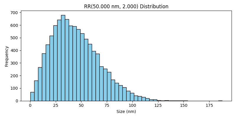
Rosin-Rammler Distribution#

The RosinRammler class generates particle sizes using the Rosin-Rammler distribution, which is commonly used to describe the size distribution of powders and granular materials. It provides a skewed distribution where most particles are within a specific range, but some larger particles may exist.

../_images/RosinRammler.png
class RosinRammler(characteristic_value, spread, cutoff=None)[source]#

Bases: Base

Rosin Rammler particle size distribution.

This class implements the Rosin Rammler distribution, which is mathematically equivalent to a Weibull distribution parameterized by a scale parameter d (here characteristic_value) and a shape parameter k (here spread).

The cumulative distribution function is

\[F(x) = 1 - \exp\!\left(-\left(\frac{x}{d}\right)^k\right),\]

where x is the sampled property (typically a diameter), d is the characteristic property (scale) and k controls the distribution width.

Hard cutoff and truncation#

When cutoff is provided, sampling is performed from the truncated distribution conditional on

\[X \ge x_{\mathrm{cut}}.\]

Operationally, this is not rejection sampling. Instead, truncation is implemented by remapping uniform random numbers from [0, 1) to the CDF interval [F(cutoff), 1) and applying the standard inverse CDF transform.

This provides an efficient way to emulate an idealized size selection step. If you interpret the cutoff as a physical removal of particles below the cutoff, you can use survival_fraction_above() to compute the concentration multiplier consistent with the same distribution.

param characteristic_value:

Scale parameter d with length units. In many applications this is a characteristic diameter.

type characteristic_value:

TypedUnit.units.AnyUnit

param spread:

Shape parameter k. Must be strictly positive.

type spread:

float

param cutoff:

Optional hard minimum value with the same units as characteristic_value. If provided, generated samples satisfy x >= cutoff by construction.

type cutoff:

TypedUnit.units.AnyUnit | None

Notes

The Rosin Rammler model is often used for particulate materials. In biological nanoparticle contexts it can be a convenient phenomenological model, but you should verify that the tail behavior is realistic for the application, especially when applying strong cutoffs.

apply_cutoff(cutoff, reduce_concentration_consistently=True)[source]#

Return a truncated Rosin Rammler distribution and an optional concentration multiplier.

This is a convenience method that supports two distinct operations.

  1. Truncating the distribution for sampling The returned distribution samples from the conditional law X | X >= cutoff.

  2. Optionally updating population concentration consistently If you interpret the cutoff as a physical removal of particles, the appropriate concentration multiplier is the survival fraction P(X >= cutoff) computed from the same distribution.

Parameters:
  • cutoff (AnyUnit) – Hard minimum value used to define the truncated sampling distribution.

  • reduce_concentration_consistently (bool) – If True, return the survival fraction P(X >= cutoff) as the concentration multiplier. If False, return 1.0 as the multiplier.

Returns:

truncated_distribution is a new RosinRammler instance with the same scale and shape but with cutoff set.

concentration_multiplier is:
  • P(X >= cutoff) if reduce_concentration_consistently is True

  • 1.0 otherwise

Return type:

truncated_distribution, concentration_multiplier

Examples

Sample truncation only:

rr_truncated, _ = rr.apply_cutoff(30 * ureg.nanometer, reduce_concentration_consistently=False)

Truncation plus concentration update:

rr_truncated, multiplier = rr.apply_cutoff(30 * ureg.nanometer, reduce_concentration_consistently=True)
population.particle_count *= multiplier
population.diameter = rr_truncated
cdf(x)[source]#

Evaluate the cumulative distribution function at x.

Parameters:

x (AnyUnit) – Quantity with the same dimensionality as characteristic_value.

Returns:

CDF value in the interval [0, 1].

Return type:

float

Raises:

ValueError – If spread is not strictly positive.

characteristic_value: AnyUnit#
cutoff: AnyUnit | None = None#
generate(n_samples)#

Generate a distribution of scatterer diameters.

Parameters:

n_samples (AnyUnit)

get_pdf(x_min=0.1, x_max=2.0, n_samples=100)[source]#

Return x values and the probability density function.

Without cutoff, the Rosin Rammler PDF is

\[f(x) = \frac{k}{d}\left(\frac{x}{d}\right)^{k-1} \exp\!\left(-\left(\frac{x}{d}\right)^k\right).\]

With cutoff, this method returns the truncated PDF for x >= cutoff:

\[\begin{split}f_{\mathrm{trunc}}(x) = \begin{cases} \frac{f(x)}{P(X \ge cutoff)} & x \ge cutoff, \\ 0 & x < cutoff. \end{cases}\end{split}\]
Parameters:
  • x_min (float) – Lower bound factor relative to characteristic_value.

  • x_max (float) – Upper bound factor relative to characteristic_value.

  • n_samples (int) – Number of points used for the x grid.

Returns:

x is a 1D array with length units. pdf is a 1D NumPy array of density values.

Return type:

x, pdf

spread: float#
survival_fraction_above(cutoff)[source]#

Compute the survival fraction above a cutoff, P(X >= cutoff).

This quantity is the natural concentration multiplier if you interpret the cutoff as physically removing all particles smaller than cutoff from an otherwise unchanged distribution.

For the Rosin Rammler distribution,

\[P(X \ge x_{\mathrm{cut}}) = \exp\!\left(-\left(\frac{x_{\mathrm{cut}}}{d}\right)^k\right).\]
Parameters:

cutoff (AnyUnit) – Hard minimum value with length units.

Returns:

Survival fraction in [0, 1].

Return type:

float

Raises:

ValueError – If spread is not strictly positive.

Parameters:
  • characteristic_value (AnyUnit)

  • spread (float)

  • cutoff (AnyUnit | None)

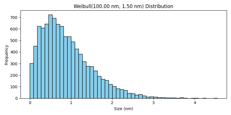
Weibull Distribution#

The Weibull class generates particle sizes according to the Weibull distribution. This distribution is flexible and can model various types of particle size distributions, ranging from light-tailed to heavy-tailed distributions, depending on the shape parameter.
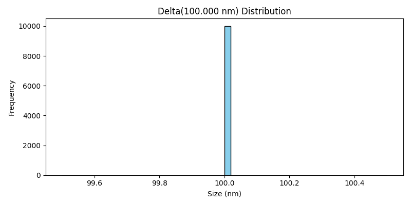
../_images/Weibull.png
class Weibull(shape, scale)[source]#

Bases: Base

Represents a Weibull distribution for particle properties.

The Weibull distribution is commonly used for modeling property distributions in biological systems.

Parameters:
  • shape (AnyUnit) – The shape parameter (k), controls the skewness of the distribution.

  • scale (AnyUnit) – The scale parameter (λ), controls the spread of the distribution.

generate(n_samples)#

Generate a distribution of scatterer diameters.

Parameters:

n_samples (AnyUnit)

get_pdf(n_samples=100)[source]#

Returns the x-values and the PDF values for the Weibull distribution.

If x is not provided, a default range of x-values is generated.

Parameters:
  • x (AnyUnit, optional) – The input x-values (particle properties) over which to compute the PDF. If not provided, a range is generated.

  • n_points (int, optional) – Number of points in the generated range if x is not provided. Default is 100.

  • n_samples (int)

Returns:

The input x-values and the corresponding PDF values.

Return type:

Tuple[AnyUnit, np.ndarray]

scale: AnyUnit#
shape: AnyUnit#

Delta Distribution#

The Delta class models particle sizes as a delta function, where all particles have exactly the same size. This distribution is useful for simulations where all particles are of a fixed size, without any variation.

../_images/Delta.png
class Delta(position)[source]#

Bases: Base

Represents a delta Dirac distribution for particle properties.

In a delta Dirac distribution, all particle properties are the same, represented by the Dirac delta function:

\[f(x) = \delta(x - x_0)\]

where: - \(x_0\) is the singular particle property.

Parameters:

position (AnyUnit) – The particle property for the delta distribution in meters.

generate(n_samples)#

Generate a distribution of scatterer diameters.

Parameters:

n_samples (AnyUnit)

get_pdf(x_min_factor=0.99, x_max_factor=1.01, n_samples=21)[source]#

Returns the x-values and the scaled PDF values for the singular distribution.

Returns:

The input x-values and the corresponding scaled PDF values.

Return type:

Tuple[AnyUnit, np.ndarray]

Parameters:
  • x_min_factor (float)

  • x_max_factor (float)

  • n_samples (int)

position: AnyUnit#

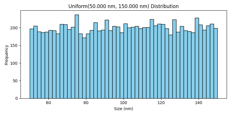
Uniform Distribution#

The Uniform class generates particle sizes that are evenly distributed between a specified lower and upper bound. This results in a flat distribution, where all particle sizes within the range are equally likely to occur.

../_images/Uniform.png
class Uniform(lower_bound, upper_bound)[source]#

Bases: Base

Represents a uniform distribution for particle properties.

The uniform distribution assigns equal probability to all particle properties within a specified range:

\[f(x) = \frac{1}{b - a} \quad \text{for} \quad a \leq x \leq b\]

where: - \(a\) is the lower bound of the distribution. - \(b\) is the upper bound of the distribution.

Parameters:
  • lower_bound (AnyUnit) – The lower bound for particle properties in meters.

  • upper_bound (AnyUnit) – The upper bound for particle properties in meters.

generate(n_samples)#

Generate a distribution of scatterer diameters.

Parameters:

n_samples (AnyUnit)

get_pdf(n_samples=100)[source]#

Returns the x-values and the PDF values for the uniform distribution.

If x is not provided, a default range of x-values is generated.

Parameters:

n_samples (int, optional) – Number of points in the generated range if x is not provided. Default is 100.

Returns:

The input x-values and the corresponding PDF values.

Return type:

Tuple[AnyUnit, np.ndarray]

lower_bound: AnyUnit#
upper_bound: AnyUnit#