A dielectric sphere in a homogeneous background

Define a finite three-dimensional refractive index field directly rather than drawing it from homogeneous random statistics. The sphere has a constant refractive index inside and is surrounded by a uniform background. The fluctuation array stores n(r) - background_refractive_index: zero outside the sphere, a constant contrast inside. The scattering problem’s background extends beyond the voxel box; the box is not an additional material boundary.

The voxel mask approximates a curved interface with a staircase boundary. Refine the spacing at fixed sphere radius and check the calculated curves before interpreting them quantitatively. BornSim uses the linearized dielectric contrast 2 * n0 * delta_n at all Born orders, rather than n_sphere**2 - n0**2. This weak-contrast example is not an exact Mie solution.

import sys

import matplotlib.pyplot as plt

from bornsim import Material, AngularSampling, Grid, Solver, Source, Sphere, StructuredMedium
from bornsim.units import ureg

Build a spherical refractive index mask

Use voxel-centre coordinates measured from the box centre. The background refractive index is 1.33 and the sphere refractive index is 1.34. A 150 nm radius fits inside a 480 nm box; no random statistics or generation seed are needed. The sphere is offset by 40 nm in x and 20 nm in y. Set this vector to zero for a centred sphere. Keep abs(centre[a]) + radius below half the box size on every axis to avoid clipping. Grid-aligned offsets translate the same mask.

grid = Grid(
    shape=(24, 24, 24),
    spacing=20 * ureg.nanometer,
)

sampling = AngularSampling(
    start=0 * ureg.degree,
    end=180 * ureg.degree,
    n_points=91,
    polar_samples=32,
    azimuth_samples=16,
)

structure = StructuredMedium()

background = Material(refractive_index=1.33)

sphere_material = Material(refractive_index=1.34)

structure.add_background(material=background)


sphere = Sphere(
    radius=150 * ureg.nanometer,
    material=sphere_material,
    centre=[40, 20, 0] * ureg.nanometer,
)

structure.add_structures(
    sphere,
)


sphere = Sphere(
    radius=150 * ureg.nanometer,
    material=sphere_material,
    centre=[-100, 0, -20] * ureg.nanometer,
)

structure.add_structures(
    sphere,
)

volume = structure.to_volume(
    grid=grid,
)

Inspect the medium in 3D

Inspect the actual finite input sample with physical spatial axes. The gallery embeds an interactive volume; drag to rotate and scroll to zoom. Level surfaces interpolate the sampled staircase interface.

medium_figure = volume.plot_3d(
    mode="volume",
    field="refractive_index",
    opacity_scale="increasing",
)

if "--no-browser" not in sys.argv:
    medium_figure.show(renderer="browser")

Compute coherent scattering through three Born orders

A single-volume result reports differential scattering as a cross section divided by the entire voxel-box volume. Multiplying by that physical volume recovers a differential cross section, which avoids treating the empty background portion of the box as part of an intrinsic transport coefficient.

source_configuration_1 = Source(wavelength=633 * ureg.nanometer)

solver = Solver(
    source=source_configuration_1,
    sampling=sampling,
    order=3,
)

result = solver.solve(
    target=volume,
)

Three-dimensional phase function

The solve above sampled the fixed volume over output directions and separate integration nodes. It supplies the solid-angle normalization directly. The normalized surface retains each azimuth, including interference between structures. Its radius is a probability density per steradian, not a spatial coordinate. No realization or azimuth averaging is applied to the 3D view. Check polar and azimuth quadrature refinement for quantitative calculations.

phase_figure = result.plot_phase_function(
    view="3d",
)

if "--no-browser" not in sys.argv:
    phase_figure.show(renderer="browser")

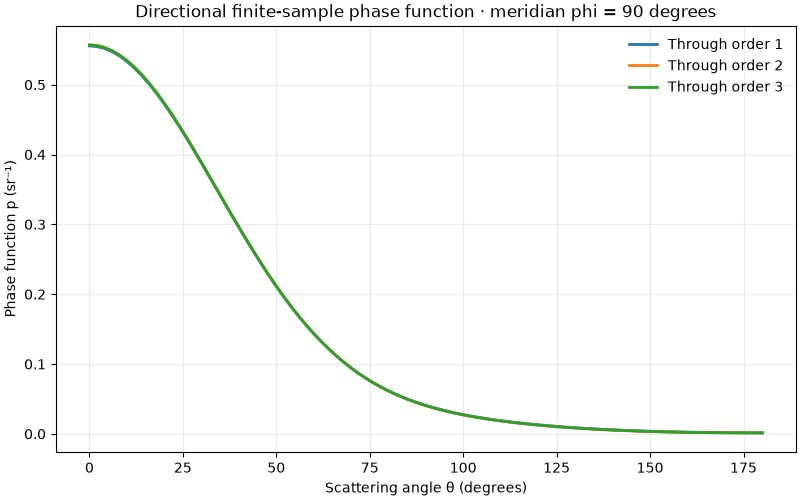
Select a physical meridian

Select the sampled phi = 90 degree plane without averaging or interpolation. The curve keeps the full solve’s solid-angle normalization.

meridian = result.meridian(azimuth=90 * ureg.degree)

meridian.plot_phase_function()

plt.show()