Layers and scatterers with numerical random fluctuations

Compose finite slabs and shaped inclusions using absolute refractive indices. Later regions replace earlier ones where they overlap. Add a seeded Whittle–Matérn fluctuation field over the complete structure, then solve numerically. The background outside the voxel box stays homogeneous. This is a finite sample with edges, not an infinite planar stack calculation.

All Born orders retain the linearized contrast 2*n0*delta_refractive_index. The smoothness convention is x=sqrt(2*nu)*r/ell; probability statistics remain Gaussian. The sampled structured volume records its fluctuation statistics and seed as provenance.

from bornsim.medium.random_medium import WhittleMaternMedium

import sys

import matplotlib.pyplot as plt
import numpy as np

from bornsim import Directions, Grid, Layer, Solver, Source, Sphere, StructuredMedium
from bornsim.units import ureg

grid = Grid.from_extent(
    shape=(16, 16, 16),
    extent=(400, 400, 400) * ureg.nanometer,
)

structure = StructuredMedium()

structure.add_background(refractive_index=1.33)

layer = Layer.from_center_and_thickness(
    centre=(0, 0, -100) * ureg.nanometer,
    thickness=200 * ureg.nanometer,
    refractive_index=1.335,
)

layer_2 = Layer.from_center_and_thickness(
    centre=(0, 0, 100) * ureg.nanometer,
    thickness=200 * ureg.nanometer,
    refractive_index=1.34,
)

sphere = Sphere(
    radius=7e-08 * ureg.meter,
    refractive_index=1.345,
    centre=(0, 0, 5e-08) * ureg.meter,
)

structure.add_structures(
    layer,
    layer_2,
    sphere,
)

structured = structure.to_volume(
    grid=grid,
)

statistics = WhittleMaternMedium(
    refractive_index_std=0.002,
    correlation_length=5e-08 * ureg.meter,
    smoothness=1.5,
    background_refractive_index=1.33,
)

structure_with_fluctuations = StructuredMedium()

structure_with_fluctuations.add_background(refractive_index=1.33)

structure_with_fluctuations.add_structures(
    layer,
    layer_2,
    sphere,
)

structure_with_fluctuations.add_fluctuations(medium=statistics)

combined = structure_with_fluctuations.to_volume(
    grid=grid,
    seed=42,
)

Inspect the structured medium in 3D

Inspect the deterministic layers and sphere before adding fluctuations. Drag to rotate and scroll to zoom in the embedded browser volume.

medium_figure = structured.plot_3d(
    mode="volume",
    field="refractive_index",
    opacity_scale="increasing",
)

if "--no-browser" not in sys.argv:
    medium_figure.show(renderer="browser")

Inspect the combined medium in 3D

This interactive volume shows the sampled refractive index used by the solver, including the same seeded Matérn fluctuations as the scattering curves. Regions with higher refractive index are more opaque; opacity is a display setting.

medium_figure = combined.plot_3d(
    mode="volume",
    field="refractive_index",
    opacity_scale="increasing",
)

if "--no-browser" not in sys.argv:
    medium_figure.show(renderer="browser")

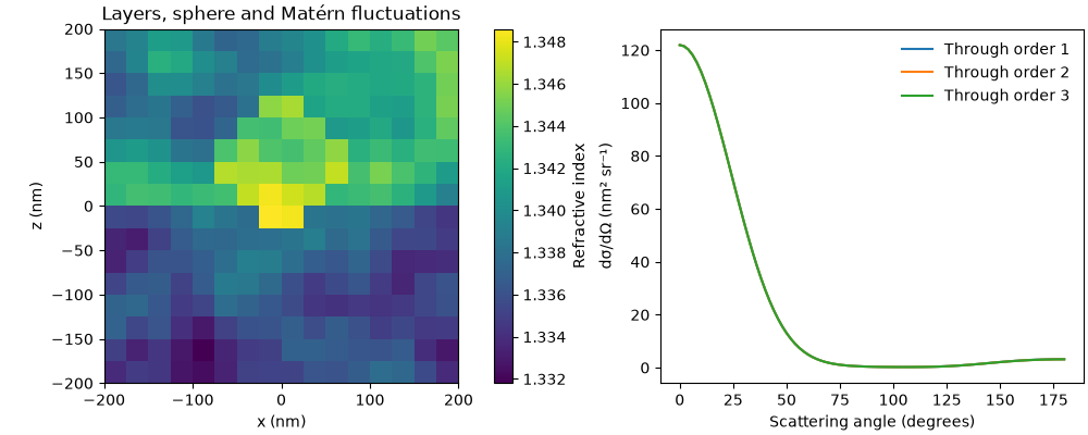
Scattering curves and a diagnostic cross-section

The slice checks exact voxel values after exploring the full volumes above.

figure, axes = plt.subplots(1, 2, figsize=(10, 4), layout="constrained")

image = axes[0].imshow(
    combined.refractive_index[:, grid.shape[1] // 2, :].T,
    origin="lower",
    extent=(-200, 200, -200, 200),
    cmap="viridis",
)

axes[0].set(xlabel="x (nm)", ylabel="z (nm)", title="Layers, sphere and Matérn fluctuations")

figure.colorbar(image, ax=axes[0], label="Refractive index")

source_configuration_1 = Source(wavelength=633 * ureg.nanometer)

solver = Solver(
    source=source_configuration_1,
    order=3,
)

angles = np.linspace(0, 180, 91) * ureg.degree

directions = Directions.from_angles(
    polar_angles=angles,
    azimuth_angles=0 * ureg.degree,
)

result = solver.solve(
    target=combined,
    sampling=directions,
)

cross_section = result.differential_cross_section.to("nanometer**2 / steradian")

for order, curve in enumerate(cross_section.magnitude, start=1):
    axes[1].plot(
        angles.to("degree").magnitude,
        curve,
        label=f"Through order {order}",
    )

axes[1].set(xlabel="Scattering angle (degrees)", ylabel="dσ/dΩ (nm² sr⁻¹)")

axes[1].legend(frameon=False)

plt.show()