Convergence of solid-angle quadrature

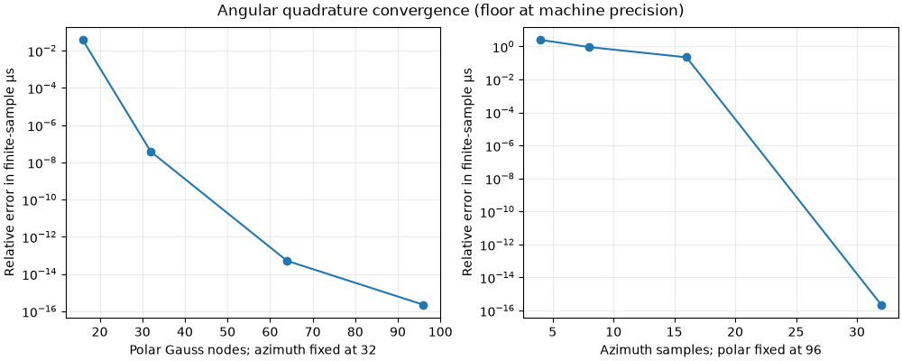
Hold the random volumes, Born order, and voxel grid fixed while increasing polar Gauss-Legendre nodes and uniform azimuth samples. Plot angles are independent of the integration nodes: adding points to an angular plot does not refine the integral. The finest calculation is a numerical reference, not an exact solution, and both quadrature axes need checking independently.

from bornsim.medium.random_medium import GaussianMedium

import sys

import matplotlib.pyplot as plt
import numpy as np

from bornsim import EnsembleSampling, AngularSampling, Grid, Solver, Source
from bornsim.units import ureg

medium = GaussianMedium(
    refractive_index_std=0.001,
    correlation_length=600 * ureg.nanometer,
    background_refractive_index=1.33,
)

source_configuration_1 = Source(wavelength=400 * ureg.nanometer)

solver = Solver(
    source=source_configuration_1,
    order=1,
)

grid = Grid(
    shape=(6, 6, 6),
    spacing=300 * ureg.nanometer,
)

ensemble_sampling = EnsembleSampling(
    realizations=2,
    seed=42,
)

options = dict(
    grid=grid,
    ensemble_sampling=ensemble_sampling,
)

reference_sampling = AngularSampling(
    angles=[0] * ureg.radian,
    polar_samples=96,
    azimuth_samples=32,
)

Refine one angular axis at a time

Identical consecutive seeds give the same volumes in every calculation. Voxel and finite-sample errors remain fixed throughout this comparison.

reference = solver.ensemble(
    medium=medium,
    **options,
    sampling=reference_sampling,
)

reference_mu = reference.mu_s.to("1 / meter").magnitude[0]

samples = np.array([16, 32, 64, 96])

polar_error = []

for count in samples:
    sampling = AngularSampling(
        angles=[0] * ureg.radian,
        polar_samples=int(count),
        azimuth_samples=32,
    )

    result = solver.ensemble(
        medium=medium,
        **options,
        sampling=sampling,
    )

    polar_error.append(abs(result.mu_s.to("1 / meter").magnitude[0] / reference_mu - 1))

azimuths = np.array([4, 8, 16, 32])

azimuth_error = []

for count in azimuths:
    sampling = AngularSampling(
        angles=[0] * ureg.radian,
        polar_samples=96,
        azimuth_samples=int(count),
    )

    result = solver.ensemble(
        medium=medium,
        **options,
        sampling=sampling,
    )

    azimuth_error.append(abs(result.mu_s.to("1 / meter").magnitude[0] / reference_mu - 1))

figure, axes = plt.subplots(1, 2, figsize=(10, 4), layout="constrained")

for axis, counts, errors, label in (
    (axes[0], samples, polar_error, "Polar Gauss nodes; azimuth fixed at 32"),
    (axes[1], azimuths, azimuth_error, "Azimuth samples; polar fixed at 96"),
):
    # A floor permits plotting exact equality with the reference on a log axis.
    axis.semilogy(counts, np.maximum(errors, np.finfo(float).eps), "o-")

    axis.set(xlabel=label, ylabel="Relative error in finite-sample μs")

    axis.grid(alpha=0.25)

figure.suptitle("Angular quadrature convergence (floor at machine precision)")

plt.show()

Inspect one ensemble realization in 3D

This is the first realization (seed 42) on the calculation grid, not an ensemble average or an infinite-medium material boundary. Drag to rotate and scroll to zoom in the embedded browser view. Regions with higher refractive index are more opaque; opacity is not absorption.

preview_volume = medium.to_volume(
    grid=grid,
    seed=42,
)

medium_figure = preview_volume.plot_3d(
    mode="volume",
    field="refractive_index",
    opacity_scale="increasing",
)

if "--no-browser" not in sys.argv:
    medium_figure.show(renderer="browser")