Monte Carlo RSA - Estimator vs Percus Yevick

This example compares the partial pair correlation functions \(g_{ij}(r)\) obtained from:

1. A Monte Carlo Random Sequential Addition (RSA) packing in 3D (PackLab.monte_carlo)

2. The analytical Percus Yevick solution for a polydisperse hard sphere mixture (PackLab.analytical)

We use a two class discrete radius distribution with radii \(r = 1\) and \(r = 2\), sampled with equal number fractions. The Monte Carlo simulation is configured to enforce the target radii distribution during packing, which is useful when larger particles are rejected more often.

The workflow is:

1. Configure a periodic cubic domain, a discrete radius sampler, and RSA options

2. Run RSA and compute partial \(g_{ij}(r)\) from the resulting configuration

3. Build the matching analytical polydisperse domain and solve Percus Yevick

4. Plot Monte Carlo curves and overlay the analytical solution

import numpy as np
import matplotlib.pyplot as plt

from PackLab import ureg
from PackLab import analytical, monte_carlo, samplers

Monte Carlo RSA setup

We use a periodic cubic domain and a two radius discrete sampler.

domain = monte_carlo.MCDomain(
    length_x=60.0 * ureg.micrometer,
    length_y=60.0 * ureg.micrometer,
    length_z=60.0 * ureg.micrometer,
    use_periodic_boundaries=True,
)

sampler = samplers.Discrete(
    radii=[1.0, 2.0] * ureg.micrometer,
    weights=[0.5, 0.5],
)

options = monte_carlo.Options()
options.maximum_attempts = 2_500_000
options.maximum_consecutive_rejections = 500_000
options.target_packing_fraction = 0.24
options.minimum_center_separation_addition = 0.0
options.enforce_radii_distribution = True

estimator = monte_carlo.Estimator(
    domain=domain,
    radius_sampler=sampler,
    options=options,
    number_of_bins=6000
)

estimate_result = estimator.estimate(
    number_of_samples=200,
    maximum_pairs=30_000_000
)

mean_g = estimate_result.mean_g
std_g = estimate_result.std_g
centers = estimate_result.centers

Analytical Percus Yevick setup

We construct an analytical polydisperse domain matching the Monte Carlo mixture. The analytical domain uses Pint quantities.

particle_radii, number_fractions = sampler.to_bins()

py_domain = analytical.PYDomain(
    size=100_000 * ureg.micrometer,
    radii=particle_radii,
    volume_fraction=0.24,
    number_fractions=number_fractions,
)

# Percus Yevick solver radial frequency grid
# Because we want to plot g we need to have a large p_max to capture the oscillations at small r.
# The p_max should be at least 10 times 2 * pi/r_min, where r_min is the smallest particle radius.
p_max = 1e3 / py_domain.radii.min()
p = np.linspace(0, p_max * 5, 30_000)

solver = analytical.Solver(
    densities=py_domain.particle_densities_per_radius,
    radii=py_domain.radii,
    p=p,
)

distances = np.linspace(
    py_domain.radii.min() * 2,
    py_domain.radii.max() * 10,
    400,
)

py_result = solver.compute(distances=distances)

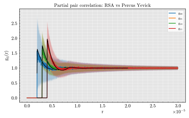
Compare Monte Carlo and analytical g_ij(r)

We plot all partial curves on the same axes and overlay the Percus Yevick result in black.

fig, ax = plt.subplots(1, 1)

K = 2
for i in range(K):
    for j in range(K):
        ax.plot(centers, mean_g[i, j], label=f"g$_{{{i}{j}}}$")
        ax.fill_between(centers, y1=mean_g[i, j] - std_g[i, j], y2=mean_g[i, j] + std_g[i, j], alpha=0.3)
        ax.plot(py_result.distances, py_result.g[i, j], color="black", linewidth=1.5)

ax.set_xlabel("r")
ax.set_ylabel(r"$g_{ij}(r)$")
ax.set_title("Partial pair correlation: RSA vs Percus Yevick")
ax.legend()
plt.show()