Propagation constant: DCFC

Imports

import numpy
from SuPyMode.workflow import Workflow, fiber_loader, Boundaries, BoundaryValue, DomainAlignment
from PyOptik import MaterialBank

from PyFiberModes import LP01
from PyFiberModes.fiber import load_fiber
import matplotlib.pyplot as plt

wavelength = 1550e-9
fiber_name = 'DCF1300S_33'

Generating the fiber structure

Here we define the cladding and fiber structure to model the problem

fiber_list = [
    fiber_loader.load_fiber(fiber_name, clad_refractive_index=MaterialBank.fused_silica.compute_refractive_index(wavelength))  # Refractive index of silica at the specified wavelength
]

Defining the boundaries of the system

boundaries = [
    Boundaries(right=BoundaryValue.SYMMETRIC, bottom=BoundaryValue.SYMMETRIC),
    Boundaries(right=BoundaryValue.SYMMETRIC, bottom=BoundaryValue.ANTI_SYMMETRIC)
]

Generating the computing workflow

Workflow class to define all the computation parameters before initializing the solver

workflow = Workflow(
    fiber_list=fiber_list,          # List of fiber to be added in the mesh, the order matters.
    wavelength=wavelength,          # Wavelength used for the mode computation.
    resolution=80,                  # Number of point in the x and y axis [is divided by half if symmetric or anti-symmetric boundaries].
    x_bounds=DomainAlignment.LEFT,  # Mesh x-boundary structure.
    y_bounds=DomainAlignment.TOP,   # Mesh y-boundary structure.
    air_padding_factor=1.3,
    boundaries=boundaries,          # Set of symmetries to be evaluated, each symmetry add a round of simulation
    n_sorted_mode=3,                # Total computed and sorted mode.
    n_added_mode=4,                 # Additional computed mode that are not considered later except for field comparison [the higher the better but the slower].
    debug_mode=0,                   # Print the iteration step for the solver plus some other important steps.
    auto_label=True,                # Auto labeling the mode. Label are not always correct and should be verified afterwards.
    itr_final=0.2,                  # Final value of inverse taper ratio to simulate
    n_step=70,
)

workflow.initialize_geometry()  # Initialize the geometry and plot it

workflow.run_solver()  # Run the solver to compute the modes

Plotting the geometry

workflow.geometry.plot()

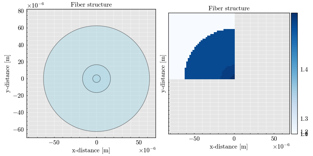
<Figure size 1000x500 with 3 Axes>

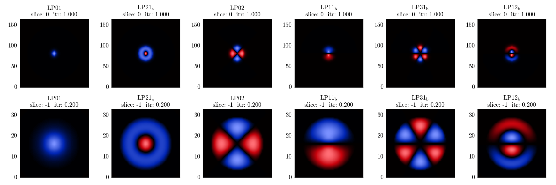
Plotting the field distribution

workflow.plot('field')

itr_list = workflow.superset.model_parameters.itr_list

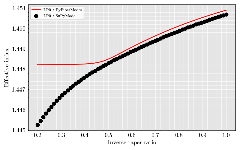
Computing the analytical values using FiberModes solver.

dcf_fiber = load_fiber(
    fiber_name=fiber_name,
    wavelength=wavelength,
    add_air_layer=True
)

Preparing the figure

figure, ax = plt.subplots(1, 1)
ax.set(
    xlabel='Inverse taper ratio',
    ylabel='Effective index',
)

pyfibermodes_mode = LP01
supymode_mode = workflow.superset.LP01

analytical = numpy.empty(itr_list.shape)
for idx, itr in enumerate(itr_list):
    _fiber = dcf_fiber.scale(factor=itr)
    analytical[idx] = _fiber.get_effective_index(mode=pyfibermodes_mode)

ax.plot(
    itr_list,
    analytical,
    label=str(pyfibermodes_mode) + ": PyFiberModes",
    linestyle='-',
    linewidth=2,
    color='red',
)

ax.scatter(
    itr_list,
    supymode_mode.index.data,
    label=str(supymode_mode) + ": SuPyMode",
    color='black',
    s=80,
    linestyle='-',
)

ax.legend()

plt.show()


# -