Propagation constant: DCFC

Imports

import numpy
from SuPyMode.workflow import Workflow, fiber_loader, Boundaries, BoundaryValue, DomainAlignment
from PyOptik import MaterialBank

import PyFiberModes
from PyFiberModes.fiber import load_fiber
from PyFiberModes.__future__ import get_normalized_LP_coupling
import matplotlib.pyplot as plt
import itertools

wavelength = 1550e-9
fiber_name = 'test_multimode_fiber'
scale_factor = 4

clad_refractive_index = MaterialBank.fused_silica.compute_refractive_index(wavelength)  # Refractive index of silica at the specified wavelength

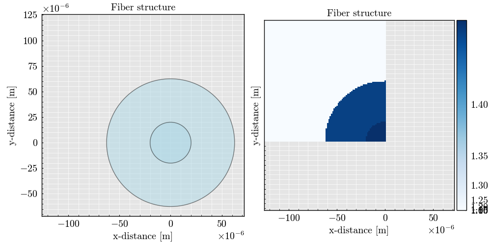
Generating the fiber structure

Here we define the cladding and fiber structure to model the problem

fiber = fiber_loader.load_fiber(fiber_name, clad_refractive_index=clad_refractive_index, remove_cladding=False)
fiber_list = [fiber]

Defining the boundaries of the system

boundaries = [
    Boundaries(right=BoundaryValue.SYMMETRIC, bottom=BoundaryValue.SYMMETRIC),
]

Generating the computing workflow

Workflow class to define all the computation parameters before initializing the solver

workflow = Workflow(
    fiber_list=fiber_list,          # List of fiber to be added in the mesh, the order matters.
    wavelength=wavelength,          # Wavelength used for the mode computation.
    resolution=180,                 # Number of point in the x and y axis [is divided by half if symmetric or anti-symmetric boundaries].
    x_bounds=DomainAlignment.LEFT,  # Mesh x-boundary structure.
    y_bounds=DomainAlignment.TOP,   # Mesh y-boundary structure.
    air_padding_factor=2.0,
    boundaries=boundaries,          # Set of symmetries to be evaluated, each symmetry add a round of simulation
    n_sorted_mode=7,                # Total computed and sorted mode.
    n_added_mode=6,                 # Additional computed mode that are not considered later except for field comparison [the higher the better but the slower].
    debug_mode=1,                   # Print the iteration step for the solver plus some other important steps.
    auto_label=True,                # Auto labeling the mode. Label are not always correct and should be verified afterwards.
    itr_final=0.4,                  # Final value of inverse taper ratio to simulate
    n_step=100
)


workflow.initialize_geometry(plot=True)  # Initialize the geometry and plot it

workflow.run_solver()  # Run the solver to compute the modes

Plotting the geometry

workflow.geometry.plot()


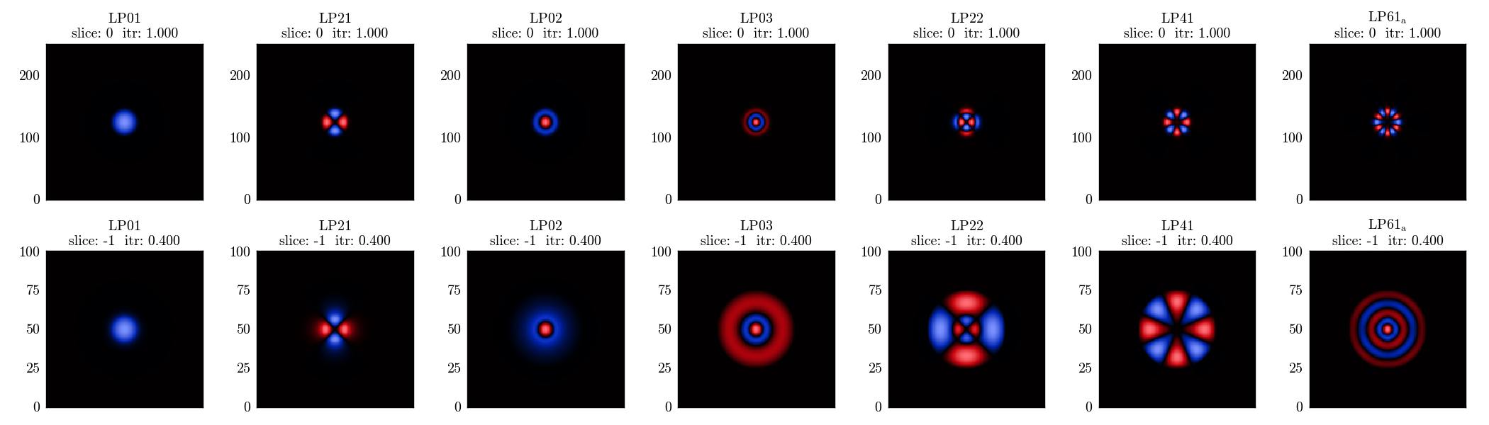
workflow.superset.label_supermodes('LP01', 'LP21', 'LP02', 'LP03', 'LP22', 'LP41')

Plotting the field distribution

workflow.superset.plot(plot_type='field')

itr_list = workflow.superset.model_parameters.itr_list

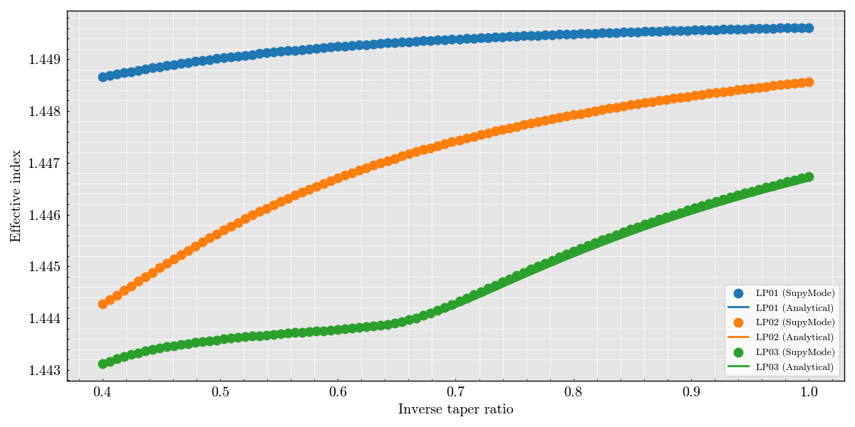
Computing the analytical values using FiberModes solver.

initial_fiber = load_fiber(
    fiber_name=fiber_name,
    wavelength=wavelength,
    add_air_layer=False
)

Preparing the figure

figure, ax = plt.subplots(1, 1, figsize=(12, 6))

ax.set(
    xlabel='Inverse taper ratio',
    ylabel='Effective index'
)


def get_index_pyfibermodes(mode, itr_list, fiber):
    analytical = numpy.empty(itr_list.shape)

    for idx, itr in enumerate(itr_list):
        tapered_fiber = fiber.scale(factor=itr)
        analytical[idx] = tapered_fiber.get_effective_index(mode=mode)

    return analytical


for idx, mode in enumerate(['LP01', 'LP02', 'LP03']):
    color = f"C{idx}"

    supymode_mode = getattr(workflow.superset, mode)
    ax.scatter(
        itr_list,
        supymode_mode.index.data,
        label=str(supymode_mode) + " (SupyMode)",
        color=color,
        s=80,
        linestyle='-'
    )

    analytical = get_index_pyfibermodes(mode=getattr(PyFiberModes, mode), itr_list=itr_list, fiber=initial_fiber)

    ax.plot(
        itr_list,
        analytical,
        label=str(mode) + " (Analytical)",
        linestyle='-',
        linewidth=2,
        color=color
    )

plt.legend()
plt.grid()
plt.show()

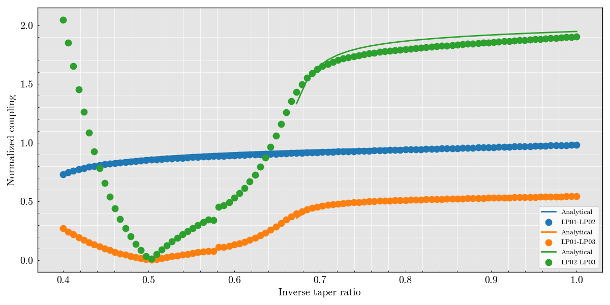
Computing the analytical values using FiberModes solver. Preparing the figure

figure, ax = plt.subplots(1, 1, figsize=(12, 6))

ax.set(
    xlabel='Inverse taper ratio',
    ylabel='Normalized coupling'
)

initial_fiber = load_fiber(
    fiber_name=fiber_name,
    wavelength=wavelength,
    add_air_layer=False
)


def get_normalized_coupling_pyfibermodes(mode_0, mode_1, itr_list, initial_fiber):
    analytical = numpy.empty(itr_list.shape)

    for idx, itr in enumerate(itr_list):
        tapered_fiber = initial_fiber.scale(factor=itr)

        analytical[idx] = get_normalized_LP_coupling(fiber=tapered_fiber, mode_0=mode_0, mode_1=mode_1)

    return analytical


for idx, (mode_0, mode_1) in enumerate(itertools.combinations(['LP01', 'LP02', 'LP03'], 2)):
    color = f"C{idx}"

    analytical = get_normalized_coupling_pyfibermodes(
        mode_0=getattr(PyFiberModes, mode_0),
        mode_1=getattr(PyFiberModes, mode_1),
        itr_list=itr_list[::2],
        initial_fiber=initial_fiber
    )

    ax.plot(
        itr_list[::2],
        abs(analytical),
        label='Analytical',
        linestyle='-',
        linewidth=2,
        color=color
    )

    simulation = getattr(workflow.superset, mode_0).normalized_coupling.get_values(getattr(workflow.superset, mode_1)) / (3.1415 * 2)

    ax.scatter(
        workflow.superset.model_parameters.itr_list,
        abs(simulation),
        color=color,
        s=80,
        linestyle='-',
        label=mode_0 + '-' + mode_1
    )

plt.legend()
plt.grid()
plt.show()

# -