Theory and numerical methods#

BornSim computes vector electromagnetic scattering from a finite refractive-index field in a uniform background. It discretizes a volume integral equation on cubic voxels, using FFT convolution to apply the background Green tensor. It does not use finite elements. The same numerical operator propagates fields in random media, layers and shaped scatterers.

This section connects the physical model to the API and to reproducible simulations. The figures are generated by the documentation examples using BornSim and Matplotlib. Their source code and calculation settings are linked beneath each figure. They illustrate specific effects; quantitative use still requires the relevant refinement checks.

Model, notation and units #

The exterior background has a real, uniform refractive index \(n_0\). A Volume stores the real scalar field

\[\delta n(\mathbf r) = n(\mathbf r)-n_0.\]

Material objects specify an absolute refractive index, rather than a contrast. StructuredMedium voxelizes the materials; GaussianMedium samples a statistical refractive index field. Both produce the same Volume representation.

Symbols and their API counterparts#
Symbol	Meaning and units	API
\(\lambda_0\)	Vacuum wavelength, m	`Source.wavelength`
\(h\), \(N_a\)	Cubic voxel width and axis counts	`Grid.spacing`, `Grid.shape`
\(n_0\), \(\delta n\)	Background refractive index and fluctuation, dimensionless	`Volume.background_refractive_index`, `Volume.delta_refractive_index`
\(M\)	Highest cumulative Born order	`Solver.order`
\(D^{[M]}\)	Differential coefficient, m⁻¹ sr⁻¹	`Result.differential`
\(\mathbf f_p^{(m)}\)	Isolated amplitude of order m, m	`Result.amplitudes`
\(p^{[M]}\)	Phase density per solid angle, sr⁻¹	`Result.phase_function`

Input lengths and angles require explicit units. Compatible quantities are converted to SI. The time convention is \(\exp(-i\omega t)\), with

\[k_0=\frac{2\pi}{\lambda_0},\qquad k=n_0k_0.\]

The constitutive model is deliberately linearized:

(1)#\[\chi(\mathbf r)=2n_0\delta n(\mathbf r),\qquad \epsilon_r(\mathbf r)=n_0^2+\chi(\mathbf r).\]

The quadratic term \(\delta n^2\) in \((n_0+\delta n)^2\) is omitted at every Born order. More iterations do not restore it. The implementation requires positive linearized permittivity and does not model absorption, magnetic contrast or tensor permittivity. Positive permittivity alone does not establish weak-contrast accuracy.

Geometry and the finite domain #

Grid gives voxel-centre coordinates and the physical box volume:

\[r_{i,a}=\left(i-\frac{N_a-1}{2}\right)h,\qquad V=N_xN_yN_zh^3.\]

The box extends half a voxel beyond its outer centres. It specifies the sampled contrast support; it is not an additional material interface. Outside it, the contrast is zero and the background continues indefinitely. A uniform refractive index inclusion that fills the box nevertheless has an interface where its contrast ends.

For a shape centre \(\mathbf c\) and proper rotation matrix \(R\), local coordinates are \(\mathbf u=R^T(\mathbf r-\mathbf c)\). Rotation input, handedness, composition, and the row-vector implementation convention are defined by bornsim.rotation.Rotation. Membership rules are evaluated at voxel centres:

Shape masks in local coordinates#
Shape	Membership
Layer	\(b_{\rm lower}\le u_a<b_{\rm upper}\).
Sphere	\(\lVert\mathbf u\rVert^2\le R_s^2\).
Ellipsoid	\(\sum_a(u_a/A_a)^2\le1\); \(A_a\) are semi-axis radii.
Box	\(\|u_a\|\le L_a/2\) on every axis; \(L_a\) are full lengths.
Cylinder	\(\|u_a\|\le H/2\) and \(\sum_{b\ne a}u_b^2\le R_s^2\).

Translation changes the centre. Rotation acts about the centre by default; an explicit world-space pivot also rotates the centre. Transforms return new immutable shapes and retain their shared Material.

With overlap="replace", ordered masks \(\mathcal M_j\) apply

\[\begin{split}n^{(j)}(\mathbf r)= \begin{cases} n_j,&\mathbf r\in\mathcal M_j,\\ n^{(j-1)}(\mathbf r),&\text{otherwise}. \end{cases}\end{split}\]

Earlier regions win with "preserve"; "error" rejects shared voxel centres. These are voxel-mask decisions, not continuous intersection tests. For a random background, \(n^{(0)}=n_0+\delta n_{\rm bg}\); structures replace that field inside their selected masks. Indices are not added.

Geometry outside the box is clipped, optionally with a warning. Curved interfaces have staircase boundaries, with no subvoxel averaging. Layers have finite lateral extent and edge scattering. The propagation background remains uniform; there is no layered-background Green function or transfer-matrix solver.

From Maxwell’s equation to Born orders #

The vector wave equation in this model is

\[\nabla\times\nabla\times\mathbf E-k^2\mathbf E =k_0^2\chi\mathbf E.\]

For \(r>0\), the outgoing background Green tensor is

\[\mathbf G(\mathbf r)= \left(\mathbf I+\frac{\nabla\nabla}{k^2}\right) \frac{e^{ikr}}{4\pi r}.\]

Define the propagation operator

\[(\mathcal K\mathbf s)(\mathbf r) =k_0^2\int_V\mathbf G(\mathbf r-\mathbf r') \mathbf s(\mathbf r')\,d^3r'.\]

The volume integral equation is \(\mathbf E=\mathbf E_{\rm inc}+\mathcal K(\chi\mathbf E)\). BornSim computes isolated field terms, followed by cumulative amplitudes:

(2)#\[\mathbf E_p^{(0)}=\mathbf e_p e^{ikz},\qquad \mathbf E_p^{(m)}=\mathcal K(\chi\mathbf E_p^{(m-1)}),\qquad \mathbf E_p^{[M]}=\sum_{m=0}^{M}\mathbf E_p^{(m)}.\]

The incident direction is +z. The transverse x and y polarizations are solved separately and their intensities receive equal weights. First-order scattering uses the incident field inside the contrast. Each later amplitude term uses one additional internal propagation interaction. order=3 retains the first three amplitude terms; it is neither a mesh-refinement level nor three independent samples.

First-order Born approximation #

Replace the internal field in the scattering integral by the incident field: \(\mathbf E(\mathbf r')\approx\mathbf E_{\rm inc}(\mathbf r')\). The resulting first-order scattered field is

(3)#\[\mathbf E_{\rm sc}^{(1)}(\mathbf r) =k_0^2\int_V\mathbf G(\mathbf r-\mathbf r') \chi(\mathbf r')\mathbf E_{\rm inc}(\mathbf r')\,d^3r',\qquad \mathbf E^{[1]}=\mathbf E_{\rm inc}+\mathbf E_{\rm sc}^{(1)}.\]

This retains one scattering interaction. Contributions from different positions still interfere as complex amplitudes. Its accuracy requires the scattered field to perturb the internal illumination only weakly; small refractive index contrast alone is insufficient for a thick sample with appreciable accumulated phase. BornSim uses the linearized contrast in (1) at every order.

Discrete Green interactions and open boundaries #

Off-diagonal voxel interactions use midpoint quadrature, \(k_0^2h^3\mathbf G(\mathbf r_i-\mathbf r_j)\). The singular diagonal uses an equal-volume spherical self cell, with \(a=(3h^3/(4\pi))^{1/3}\):

(4)#\[\mathbf K_{\rm self}= \frac{k_0^2}{3k^2} \left[2\left(e^{ika}(1-ika)-1\right)-1\right]\mathbf I.\]

The final minus one includes the longitudinal contact contribution \(-\mathbf I\delta(\mathbf r)/(3k^2)\). This convention is an approximation to the singular cubic-cell integral, not its exact value. The implementation uses a small-\(ka\) expansion to avoid cancellation.

FFT convolution doubles each grid dimension, zero-pads the source and crops the result back to the physical box. This applies the finite discrete convolution without wrap-around electromagnetic interactions. Its padding has a different purpose from the periodic box used to synthesize random fields. The implemented kernel is visible in bornsim.green; independent matrix comparisons are described in Development and releases.

Amplitudes, interference and cross sections #

For observation direction \(\hat{\mathbf s}\), the isolated order-m far-field amplitude of polarization p is

\[\mathbf f_p^{(m)}(\hat{\mathbf s})= \frac{k_0^2}{4\pi} (\mathbf I-\hat{\mathbf s}\hat{\mathbf s}^{T}) \int_V\chi(\mathbf r)\mathbf E_p^{(m-1)}(\mathbf r) e^{-ik\hat{\mathbf s}\cdot\mathbf r}\,d^3r.\]

The transverse projector removes the far-field longitudinal component. Amplitudes have units of metres. The cumulative differential cross section is

(5)#\[\frac{d\sigma^{[M]}}{d\Omega} =\frac12\sum_{p=x,y} \left\lVert\sum_{m=1}^{M}\mathbf f_p^{(m)}\right\rVert^2, \qquad D^{[M]}=\frac1V\frac{d\sigma^{[M]}}{d\Omega}.\]

For two amplitude terms, the cross term is \(2\operatorname{Re}(\mathbf f^{(1)*}\cdot\mathbf f^{(2)})\). It can have either sign. Summing isolated intensities therefore cannot reconstruct the coherent cumulative intensity. Interference occurs within each incident polarization; the two incident polarizations are averaged incoherently.

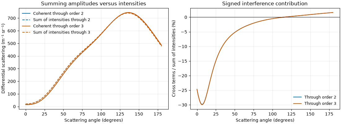
Simulated cumulative and isolated Born intensities, with a signed interference contribution. — Numerical Born terms for one seeded finite volume. The signed difference between coherent scattering and the sum of isolated intensities displays the interference contribution. Simulation code.#

Result stores \(D^{[M]}\) in m⁻¹ sr⁻¹. result.differential_cross_section multiplies it by the stored physical box volume to recover m² sr⁻¹. The volume includes background voxels. These finite-sample coefficients are not automatically intrinsic infinite-medium transport coefficients.

First-order structure and directional asymmetry #

At first order, the amplitude samples the spatial Fourier transform of the contrast at the scattering wavevector

\[\mathbf q=k(\hat{\mathbf s}-\hat{\mathbf z}),\qquad |\mathbf q|=2k\sin(\theta/2),\qquad \mathbf f_p^{(1)}\propto (\mathbf I-\hat{\mathbf s}\hat{\mathbf s}^{T})\mathbf e_p \int_V\chi(\mathbf r)e^{-i\mathbf q\cdot\mathbf r}\,d^3r.\]

Translating a completely contained scatterer by \(\mathbf d\) multiplies this amplitude by \(e^{-i\mathbf q\cdot\mathbf d}\), whose modulus is one. Intensity is unchanged. On a voxel grid, integer-voxel translations preserve the mask exactly; arbitrary shifts can change voxelization.

For two identical, nonoverlapping copies separated by \(\mathbf d\), the first-order intensity acquires the factor

\[\left|1+e^{-i\mathbf q\cdot\mathbf d}\right|^2 =2+2\cos(\mathbf q\cdot\mathbf d).\]

Transverse separation introduces azimuth dependence. Thus a translated single sphere can have the same intensity as a centred sphere, while a pair generally has a directionally asymmetric pattern. This simple factor describes first order; higher orders also include interactions between particles.

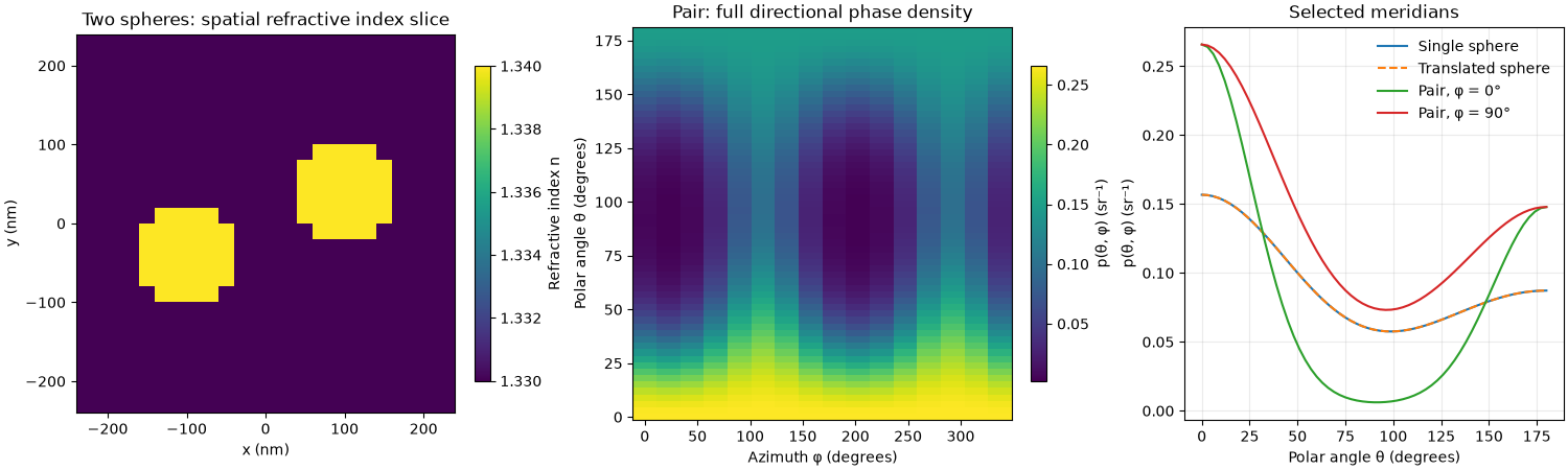
Two voxelized spheres, their azimuth-dependent phase density, and selected meridians compared with a translated single sphere. — First-order numerical simulations at 633 nm vacuum wavelength, with 20 nm voxels and refractive index 1.34 in a 1.33 background. Integer-voxel translation leaves the single-sphere curve unchanged, while two spheres produce different meridians. The simulation asserts translation invariance. Simulation code.#

Drag to rotate the pair’s full phase-density surface, which retains every sampled azimuth. Its radius is a density in direction space, not a position in the medium.

Solid-angle normalization and angular sampling #

Directions are \(\hat{\mathbf s}=(\sin\theta\cos\phi, \sin\theta\sin\phi,\cos\theta)\), with \(d\Omega=\sin\theta\,d\theta\,d\phi\). For each cumulative Born order,

(6)#\[\mu_s=\int_{4\pi}D\,d\Omega,\qquad g=\frac{\int_{4\pi}D\cos\theta\,d\Omega}{\mu_s},\qquad \mu_s'=\int_{4\pi}D(1-\cos\theta)\,d\Omega=\mu_s(1-g).\]

When \(\mu_s>0\), the phase function is \(p=D/\mu_s\), with \(\int_{4\pi}p\,d\Omega=1\). It is a density per steradian, not per polar angle. At zero scattering, phase normalization is undefined and anisotropy is NaN; the reduced coefficient is zero, using the zero-scattering limit of the moment integral.

AngularSampling separates output angles from integration accuracy. If \(u=\cos\theta\), Gauss–Legendre nodes \(u_i\) and weights \(w_i\) combine with uniform azimuths \(\phi_j=2\pi j/N_\phi\):

\[\int_{4\pi}F\,d\Omega\approx \frac{2\pi}{N_\phi}\sum_j\sum_i w_i F(\arccos u_i,\phi_j).\]

angles selects output polar angles; polar_samples selects quadrature nodes; azimuth_samples sets both output and integration azimuths. Increasing output angles alone does not refine the solid-angle integral.

Full results retain (order, polar angle, azimuth) data. No azimuth average is implicit. result.meridian(azimuth=...) selects a sampled angle exactly, or explicitly the nearest sample, without interpolation. It retains the full solve’s normalization. result.azimuth_average() instead computes

\[\overline D(\theta)=\frac1{N_\phi}\sum_jD(\theta,\phi_j).\]

The same operation on phase densities retains their full normalization. For an axisymmetric distribution only, the polar-angle density is \(2\pi p(\theta)\sin\theta\). For a general distribution it is \(\sin\theta\int_0^{2\pi}p(\theta,\phi)\,d\phi\). A single meridian is insufficient to infer that marginal or \(\mu_s\). Consequently solve_cut does not infer integrated coefficients from a cut.

Random fields and Whittle–Matérn covariance #

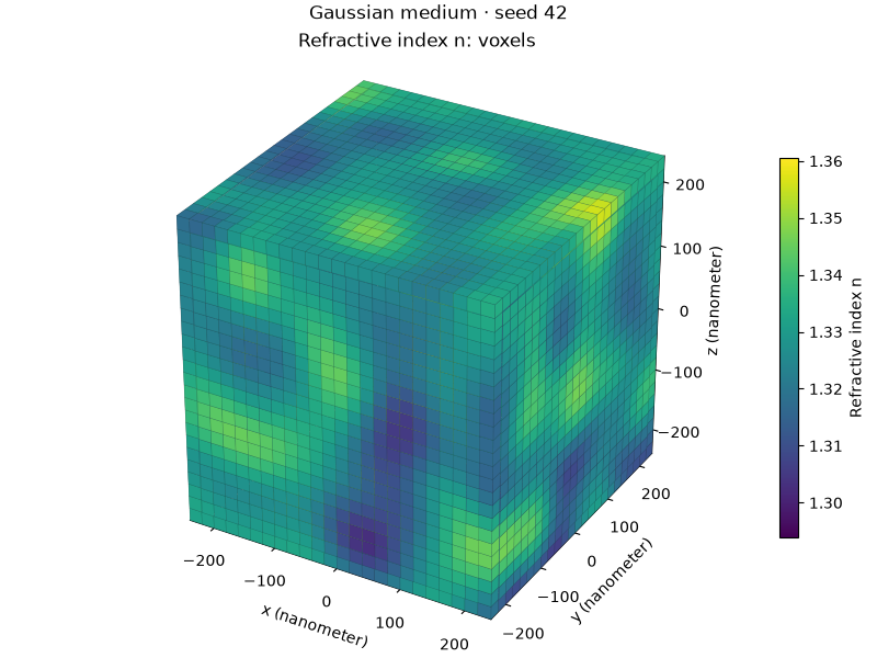
GaussianMedium describes a stationary isotropic Gaussian probability field with ensemble mean zero and point variance \(\sigma_n^2\). The covariance describes spatial correlations: \(C_n(r)=\langle\delta n(\mathbf x)\delta n(\mathbf x+\mathbf r)\rangle\). Choosing exponential or Matérn covariance does not change the Gaussian one-point probability distribution.

BornSim’s length and smoothness convention is

\[\begin{split}C_n(r)=\begin{cases} \sigma_n^2 e^{-r^2/(2\ell^2)},&\text{Gaussian},\\ \sigma_n^2 e^{-r/\ell},&\text{exponential},\\ \displaystyle\sigma_n^2\frac{2^{1-\nu}}{\Gamma(\nu)} x^\nu K_\nu(x),\quad x=\sqrt{2\nu}\,r/\ell,&\text{Matérn}. \end{cases}\end{split}\]

Here \(C_n(0)=\sigma_n^2\), \(\nu>0\) and \(K_\nu\) is the modified Bessel function. Exponential covariance is Matérn with \(\nu=1/2\). For \(\nu=3/2\), \(C_n(r)/\sigma_n^2=(1+\sqrt3r/\ell)e^{-\sqrt3r/\ell}\). Equal length parameters do not make the different covariance models identical.

With \(\Phi_n(\mathbf q)=\int C_n(\mathbf r)e^{-i\mathbf q\cdot\mathbf r}d^3r\), the dimensionless spectral shapes used for synthesis are

\[\begin{split}w(q)=\begin{cases} e^{-q^2\ell^2/2},&\text{Gaussian},\\ (1+q^2\ell^2)^{-2},&\text{exponential},\\ (1+q^2\ell^2/(2\nu))^{-\nu-3/2},&\text{Matérn}. \end{cases}\end{split}\]

Synthesis uses a periodic box of shape \((2N_x,2N_y,2N_z)\) at spacing h, then retains the first half of each axis. For independent standard normal samples \(\xi\), NumPy FFT normalization gives

\[\delta n_j=\sigma_n\operatorname{Re}\left[ \operatorname{IFFT}\left(\operatorname{FFT}(\xi) \sqrt{w/\overline w}\right)\right]_j, \qquad \overline w=\text{mean of the discrete weights}.\]

Normalization sets the expected point variance. Each realization’s spatial mean and variance fluctuate; samples are not recentered or rescaled and the DC mode is retained. The expected discrete normalized covariance is \(\operatorname{IFFT}(w/\overline w)\). Spectral truncation and finite box size change its relationship to the continuum covariance.

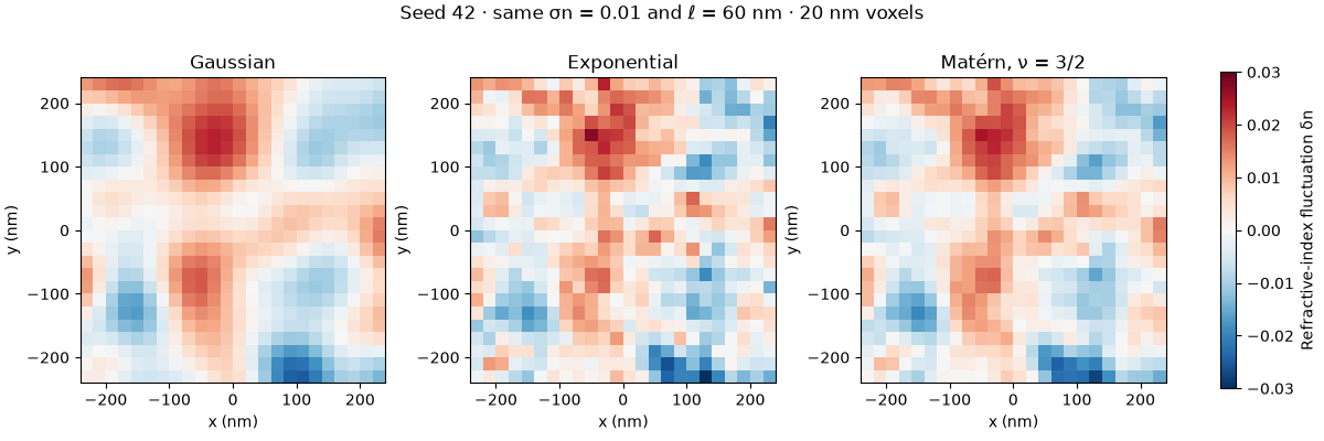
Seeded refractive index slices from Gaussian, exponential and Matérn covariance fields with a shared color scale. — Seeded numerical refractive index slices at equal standard deviation and length parameter. Covariance changes spatial texture, not the Gaussian probability law. Simulation code.#

Empirical covariance with standard-error bars from 32 independent fields, compared with discrete synthesis and continuum predictions. — Covariance estimates from 32 independent realizations. Error bars describe uncertainty across realizations. Dashed curves predict discrete synthesis; dotted curves show the continuum convention. Samples are not demeaned. Differences from continuum curves can persist beyond sampling uncertainty.#

At first order, random-field covariance connects to scattering through the Fourier transform of the finite windowed field. For a sample window W,

\[\left\langle\left|\int W(\mathbf r)\delta n(\mathbf r) e^{-i\mathbf q\cdot\mathbf r}d^3r\right|^2\right\rangle =\iint W(\mathbf r)W(\mathbf r')C_n(\mathbf r-\mathbf r') e^{-i\mathbf q\cdot(\mathbf r-\mathbf r')}d^3r\,d^3r'.\]

The finite window matters even after averaging many realizations. Changing the box size and changing the number of samples therefore address different errors. Infinite-medium first-order formulas are retained only as test references; the public solver computes finite-volume Born calculations.

Ensembles and uncertainty #

A fixed structure or a single realized random volume uses solve. An ensemble uses independent random fields or random backgrounds generated from the ordered seeds in EnsembleSampling. Duplicate seeds are rejected because repeated fields do not provide independent sampling uncertainty.

For R independent realization intensities \(D_r\),

\[\widehat D=\frac1R\sum_rD_r,\qquad \operatorname{SE}(\widehat D)= \sqrt{\frac{\sum_r(D_r-\widehat D)^2}{R(R-1)}}.\]

The amplitudes interfere coherently within each realization. The ensemble then averages intensities, never random amplitudes. For one realization, error is unknown and reported as NaN. Integrated ensemble anisotropy is the ratio of averaged angular moments, not an average of per-realization ratios.

Azimuth averaging introduces correlated angular samples. BornSim computes each realization’s azimuth average before estimating its standard error:

\[\operatorname{Var}\left(\frac1{N_\phi}\sum_jD_j\right) =\frac1{N_\phi^2}\sum_{j,l}\operatorname{Cov}(D_j,D_l).\]

Averaging directional error bars or treating directions as independent would omit those covariances. Phase plots do not infer uncertainty in the ratio \(D/\mu_s\) from intensity errors alone; its uncertainty also involves numerator–denominator covariance.

Resolution, convergence and interpretation #

The Born expansion is a Neumann series for \(\mathcal A=\mathcal K\chi\). For a fixed finite discrete matrix, spectral radius \(\rho(\mathcal A)<1\) is sufficient for convergence. Decreasing observed field norms over a few orders does not establish universal convergence or discretization accuracy.

Keep the following checks separate:

What each refinement changes#
Check	Hold fixed	Assess
Reduce voxel spacing	Physical geometry and contrast	Interfaces, midpoint quadrature and Green discretization
Increase angular quadrature	Same Volume or exact seed list	Solid-angle integrals and directional resolution
Increase realization count	Grid and medium statistics	Sampling uncertainty
Increase physical sample size	Voxel spacing and statistics	Finite-window and synthesis-box effects
Increase Born order	Volume and sampling	Sensitivity to additional interaction terms

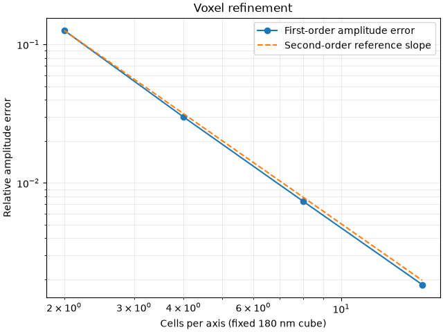
First-order amplitude error decreasing with voxel refinement for a fixed cube, compared with a second-order reference slope. — Refinement at fixed 180 nm cube size, compared with an independent exact first-order volume integral. This checks midpoint amplitude quadrature; it does not validate higher-order Green self interactions. Simulation code.#

Sampling-error bars exclude geometry, constitutive, quadrature and finite-size bias. For reproducible calculations, retain Grid, AngularSampling, Material, medium settings, EnsembleSampling and software versions. Results are immutable; archives retain their physical sample volume, arrays and provenance, but do not store the original voxel field. See Public Python API for interfaces and Examples for runnable refinement and uncertainty studies.