

Finite-sample P1 solver#
This chapter derives the boundary condition and finite-element equations
used by P1. It starts from the P1 transport model in
Transport theory and approximations, explains the meaning of every boundary quantity, and follows
the weak equation through tetrahedral assembly and power accounting.
What problem does the finite solver solve?#
The unknown \(\Phi(\mathbf r)\) is steady fluence rate inside a finite rectangular sample. The diffusion current is
In a sample with no light generated internally, conservation of radiant power gives \(\nabla\cdot\mathbf J+\mu_a\Phi=0\). Substituting Fick’s law, \(\mathbf J=-D\nabla\Phi\), produces the finite-domain equation
This equation comes from the first two angular moments of the radiative transfer equation and the P1 closure; Transport theory and approximations derives those steps. The finite sample has no point source in its interior. Illumination enters through one boundary face, and all six faces must have an explicitly selected condition.
What a Robin face represents#
A Robin condition relates the fluence on a surface to the net current through that surface. Here it represents a diffuse optical boundary: some diffuse radiation reaching the face is reflected back into the sample, some escapes, and a user may supply additional diffuse illumination entering the sample. It is a model for angularly diffuse light at a boundary, not a model of a collimated beam refracting across an interface.
The direction convention matters. The outward unit normal is \(\mathbf n\); positive \(\mathbf J\cdot\mathbf n\) means net power is leaving the sample. Define the outgoing and incoming partial currents as
Both are nonnegative irradiances in \(\mathrm{W\,m^{-2}}\). They measure the inward or outward part of the directional light flow; the net normal current is their difference, \(\mathbf J\cdot\mathbf n=J_{\mathrm{out}}-J_{\mathrm{in}}\).
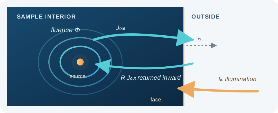
The Robin model balances outgoing diffuse current, its reflected fraction, and externally prescribed incoming diffuse current at the sample face.#
Where the Robin coefficients come from#
P1 approximates the angular radiance at the face by
Apply this expression to the two half-spheres on either side of the face. Writing \(J_n=\mathbf J\cdot\mathbf n\) and integrating over directions gives
The numerical factors come from hemisphere integration, not fitted leakage parameters. Choose the polar axis along \(\mathbf n\) and write \(\xi=\mathbf s\cdot\mathbf n\). Azimuthal integration cancels the tangential components of current. The outward integral becomes
Integrating \(-\xi L\) over \(-1<\xi<0\) gives the inward expression. Matching these integrated partial currents is a P1 boundary closure: it does not impose the exact incoming radiance separately in every direction.
Equivalently, the P1 half-range relation is
MomentRT uses the following diffuse reflection model at a face:
Here \(R\) is the effective fraction of internally outgoing diffuse partial current returned inward by the boundary. \(I_{\mathrm{in}}\) is an externally specified incoming diffuse partial-current irradiance, already coupled into the sample. Substituting this relation into the P1 half-range equations and solving for the net current gives
where
Both coefficients are dimensionless, so each term in the current condition has the same \(\mathrm{W\,m^{-2}}\) units as \(\mathbf J\cdot\mathbf n\).
The first term describes current generated by fluence inside the sample and directed outward after accounting for diffuse reflection. Its coefficient \(\beta\) decreases as \(R\) increases, so a more reflective face leaks less light for the same fluence. The second term is negative because incoming illumination points opposite to the outward normal. \(c_R\) accounts for how that incoming diffuse current couples to the P1 boundary field.
For example, the coefficients at three reflectances are:
\(R\) |
\(\beta\) |
\(c_R\) |
Interpretation |
|---|---|---|---|
0 |
1/2 |
2 |
No internal diffuse partial current is reflected. |
0.5 |
1/6 |
4/3 |
Half of the outgoing diffuse partial current returns. |
0.9 |
1/38 |
20/19 |
Most outgoing diffuse partial current returns. |
For instance, with \(R=0.5\), the boundary law becomes \(\mathbf J\cdot\mathbf n=\Phi/6-(4/3)I_{\mathrm{in}}\). With no illumination on that face, the net outward current is one sixth of its local fluence rate. The reflectance sweep example compares finite-sample fluence and escaping power for \(R=0\), \(0.5\), and \(0.9\).
The net current \(\mathbf J\cdot\mathbf n\) includes both outgoing and incoming directions, so it is not the same as the transmitted power that escapes to the outside. In this closure, the transmitted outgoing partial current is
For an unilluminated Robin face, \(I_{\mathrm{in}}=0\), so its escaping
current is \(\beta\Phi\). On an illuminated face the known incident
contribution \(2\beta I_{\mathrm{in}}\) must be removed from gross Robin
leakage to count only power transmitted outward. MomentRT applies exactly this
correction when it reports outgoing_power_by_face and escaping_power.
In the API, \(R\) is the dimensionless value
RobinBoundary(effective_reflectance=R). The name describes the role of the
parameter in this boundary model. It is not the normal-incidence Fresnel
reflectance computed from refractive indices. MomentRT has no external
refractive-index rule that converts material properties to \(R\); the
caller must select an appropriate effective diffuse coefficient.
The accepted range is \(0\le R<1\). At \(R=0\), none of the outgoing
diffuse partial current returns to the sample, and
\(\beta=1/2\), \(c_R=2\). As \(R\) approaches one, leakage tends
to zero. Use ReflectingBoundary for the separate zero-normal-current
condition \(\mathbf J\cdot\mathbf n=0\); it is not illuminated and adds
no boundary leakage or source terms to the solve.
Why this is called a Robin condition#
Inserting \(\mathbf J=-D\nabla\Phi\) into the current law gives
The name describes a mixture of a boundary value and a normal derivative. It is useful to distinguish three mathematical boundary choices:
Type |
Mathematical prescription |
Interpretation |
|---|---|---|
Dirichlet |
\(\Phi=\Phi_b\) |
Prescribes the fluence itself. |
Neumann |
\(-D\partial_n\Phi=j_b\) |
Prescribes net outward current. A reflecting face has \(j_b=0\). |
Robin |
\(D\partial_n\Phi+\beta\Phi=c_RI_{\mathrm{in}}\) |
Relates leakage to local fluence and imposed incoming light. |
MomentRT exposes the reflecting and diffuse Robin choices. It does not provide a general prescribed-fluence boundary through this API. An unilluminated open Robin face can have nonzero fluence at the actual sample surface; setting fluence to zero there would impose a different boundary model.
On an unilluminated planar face, division by \(\beta>0\) gives
Locally extrapolating the fluence linearly along the outward normal would make it vanish a distance \(z_b\) outside the sample. This is the origin of the extrapolated-boundary interpretation. The relation is a local linear extrapolation, not a statement that the physical field actually exists in an added slab of material. MomentRT imposes the Robin term on the real face; it does not enlarge the mesh by \(z_b\).
For example, at \(R=0.5\) one has \(\beta=1/6\) and \(z_b=6D\). The boundary becomes less leaky as \(R\) increases. For the illuminated top face \(z=z_{\min}\), the outward normal is \(-\mathbf e_z\) even though positive z points into the sample. The same outward-normal law is used on every face, so the incident source always enters with the correct inward sign.
What the illumination input means#
SurfaceSource.optical_power and UniformSurfaceSource.optical_power
are total diffuse optical power already entering the sample. They do not
include collimated LED propagation, specular Fresnel losses, or the design of
an illumination optic. The solver distributes this power over the configured
face and represents its incoming irradiance as \(I_{\mathrm{in}}\):
UniformSurfaceSourceuses \(I_{\mathrm{in}}=P/A\) over the entire face, where \(P\) is its specified optical power and \(A\) is face area.SurfaceSourceuses a circular top-hat spot. Triangle quadrature samples the disk; the specified power is normalized by the sampled area so its integral equals \(P\).
The face containing the source must use RobinBoundary. The other five
faces may be Robin or reflecting. The source disk must fit on its face, and
the Cartesian mesh must span the sample exactly.
Weak form: from the continuous equation to the solve#
The weak form is the continuous equation written in a way that only requires first derivatives of the unknown field. This is useful for linear finite elements, whose basis functions are continuous and piecewise linear but whose gradients can jump at tetrahedron faces.
Start with the general diffusion equation including a possible volume source \(q_0\):
Let \(v\) be any test function and multiply both sides by \(v\). On the divergence term use integration by parts, or equivalently the divergence theorem applied to \(v\mathbf J\) with \(\mathbf J=-D\nabla\Phi\):
This identity also shows why the boundary current has a plus sign on the left. Substitute \(\mathbf J\cdot\mathbf n=\beta\Phi-c_RI_{\mathrm{in}}\) on Robin faces. On reflecting faces the current is zero. With \(\partial\Omega_R\) denoting the Robin portion of the surface, the weak problem becomes
MomentRT’s finite solver has \(q_0=0\); illumination contributes only the rightmost surface integral. The Robin fluence term adds a positive boundary matrix to the left, and incoming light adds a boundary load to the right. Reflecting faces add neither term. This sign arrangement is what makes positive incoming illumination drive a positive fluence solution.
Finite-element basis and matrices#
CartesianMesh.from_sample(sample=sample, shape=(n_x, n_y, n_z)) places
nodes on the sample faces. Every Cartesian cell is split into six tetrahedra
that share one consistent body diagonal. The total number of tetrahedra is
On a tetrahedron \(e\), represent fluence by four linear basis functions:
The nodal coefficients \(\Phi_i\) are the unknowns. Linear basis gradients \(\nabla N_i\) are constant within an element. Absorption and reduced-scattering properties are evaluated at each tetrahedron centroid; that element then has constant diffusion coefficient
Choose \(v=N_j\) in the weak equation and substitute the basis expansion. The element diffusion and absorption matrices are
The mass matrix formula is the exact integral of products of linear basis functions over a tetrahedron. On a Robin boundary triangle \(f\), with area \(A_f\), the exact linear-triangle boundary matrix is
These matrices are added into a sparse global matrix. Incoming irradiance is integrated against each boundary basis function to form the load vector. Disk illumination uses a three-point triangle quadrature rule; quadrature points outside the disk receive zero irradiance. The assembled system is
More explicitly, for a global pair of nodes \(i,j\), assembly sums the contributions of every element and Robin triangle containing those nodes:
The sum notation here assumes local entries are placed at the corresponding global node indices. A reflecting triangle has no \(B^{(f)}\) or source load. MomentRT solves the sparse system with SciPy and checks the relative residual \(\lVert\mathbf A\boldsymbol\Phi-\mathbf b\rVert/ \lVert\mathbf b\rVert\) before returning the field.
For uniform illumination, \(I_{\mathrm{in}}\) is constant over each triangle. Since \(\int_fN_i\,dA=A_f/3\), its local load is exactly \(b_i^{(f)}=c_R I_{\mathrm{in}}A_f/3\).
For a disk, let \(\chi_{fq}\) be one when quadrature point \(q\) on face triangle \(f\) lies inside the disk and zero otherwise. The three quadrature points have barycentric coordinates given by the permutations of \((2/3,1/6,1/6)\) and equal weights \(1/3\). The sampled illuminated area and incoming irradiance are
The load at local node \(i\) is then
Because \(\sum_iN_i=1\), the sum of the source load entries is \(c_RP_{\mathrm{in}}\). Normalization preserves the specified incoming power even when the sampled disk differs from its geometric area \(\pi r_s^2\). Compare the reported sampled area with that geometric area and refine the footprint: conservation by normalization does not prove that the spatial distribution of illumination is resolved. If no quadrature point lands in the disk, the solver rejects the unresolved source.
After solving this sparse linear system, the fluence values are put back on the three-dimensional mesh. Within each tetrahedron, its constant gradient gives the element-centered current
The field is not smoothed across element faces or optical interfaces.
What makes the linear system well posed?#
For a real test field \(w\), the quadratic form of the continuous operator is
All three terms are nonnegative for the package’s material and boundary coefficients. For a connected sample, absorption on a region of positive volume or Robin leakage on a face of positive area controls the otherwise undetermined constant mode. This explains the positive diffusion, absorption, and boundary contributions in the assembled matrix.
A source-free, perfectly reflecting, nonabsorbing sample has a constant nullspace: any spatially constant fluence satisfies its steady equation. A nonzero net input in such a closed nonabsorbing system would accumulate energy rather than reach a steady state. The package’s illuminated face must be Robin with \(R<1\), which supplies leakage and excludes this particular degeneracy for supported illumination configurations.
Positive coefficients and a positive energy form do not by themselves guarantee nonnegative nodal values on every discretization. A discrete maximum principle also depends on the mesh and matrix structure. MomentRT reports the minimum fluence rather than clipping a negative value.
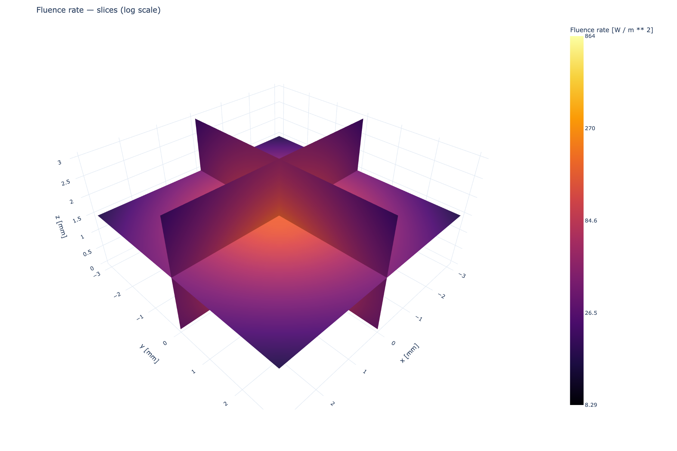
The finite-sample P1 FEM solution. These are sampled mesh planes, not smoothed reconstructions.#
One solve, step by step#
The finite workflow follows directly from the weak equation:
Define the finite sample extent and assign a background material.
Add named layers or inclusions; later structures replace earlier materials where they overlap.
Create a Cartesian mesh spanning all six sample faces. Plan the resolution around thin layers, curved interfaces, and the illumination footprint.
Select one face as the illuminated face and specify its incoming diffuse power and profile.
Assign either a Robin or reflecting condition to each face. The illuminated face must be Robin. Supply an explicit
effective_reflectancefor every Robin face.Split cells into tetrahedra, sample material coefficients at centroids, and assemble the element and boundary matrices.
Integrate the source over boundary triangles, solve the sparse system, and evaluate nodal fluence and element-centered current.
Check the linear residual, sampled source area, mesh refinement, and energy balance before interpreting the result.
import numpy as np
import MomentRT

from MomentRT import (
    CartesianMesh,
    P1,
    Material,
    RobinBoundary,
    Simulation,
    StructuredMedium,
    SurfaceSource,
    ureg,
)

material = Material(
    absorption=0.02 / ureg.millimeter,
    reduced_scattering=1.0 / ureg.millimeter,
    refractive_index=1.4,
    phase_function=MomentRT.phase_function.HenyeyGreenstein(),
)

sample = StructuredMedium(
    origin=(-4, -4, 0) * ureg.millimeter,
    size=(8, 8, 4) * ureg.millimeter,
)

sample.add_background(material=material)

mesh = CartesianMesh.from_sample(
    sample=sample,
    shape=(17, 17, 9),
)

source = SurfaceSource(
    face="z_min",
    position=np.array([0, 0, 0]) * ureg.millimeter,
    radius=1.5 * ureg.millimeter,
    wavelength=970 * ureg.nanometer,
    optical_power=1 * ureg.milliwatt,
)

boundary = RobinBoundary(effective_reflectance=0.4)

solver = P1(
    boundaries=MomentRT.Boundaries.uniform(condition=boundary),
)

simulation = Simulation(
    medium=sample,
    source=source,
    mesh=mesh,
    solver=solver,
)

result = simulation.run()
This compact homogeneous example illustrates the solver setup; the finite-sample gallery adds layered geometry and plots the computed fields.
Material sampling and interface approximation#
StructuredMedium starts with its background, then applies structures in
insertion order. Later structures replace earlier materials where they
overlap. The solver assigns material properties to an element using the
element centroid. It does not create an interface-conforming mesh. An
interface aligned with mesh planes is represented cleanly; an unaligned
planar interface or curved sphere is approximated through the centroids of
nearby elements. Refine the mesh and align important planar boundaries when
possible.
The formulation uses one continuous fluence field. MomentRT rejects internal refractive-index jumps because it does not model refraction or the associated interface jump conditions. Absorption and reduced scattering may still vary between structures.
For a perfectly contacted internal interface with equal refractive indices and no surface source, the continuous diffusion model uses
where the same oriented normal is used on both sides. The second condition comes from integrating conservation over a thin pillbox around the interface: no finite surface absorption or source remains as the pillbox thickness tends to zero. With unequal diffusion coefficients, normal gradients can jump while normal current remains continuous.
The shared nodal basis enforces continuous fluence, and the weak equation enforces current transmission in an integral sense. The computed piecewise-constant element currents need not match pointwise on individual faces of a finite mesh. Refinement is required to assess that approximation. Index mismatch requires a different interface law and is outside this continuous-fluence model.
Power accounting and verification#
The assembled balance has a direct physical interpretation. Absorption removes power in the volume, prescribed illumination supplies power through the source face, and partial current leaves through the boundaries. The reported transmitted escape removes the incident contribution from gross Robin leakage:
result.energy_balance reports these unit-bearing powers. Escaping power
on the source face is a transmitted partial current integrated over the
whole face; it is not the same as the net current through that face or a
detector reading. result.outgoing_power_by_face separates the integrated
escape by face.
The balance follows directly by choosing the constant test function \(v=1\). The gradient term vanishes, leaving
where \(c_R\) is the coefficient on the single illuminated face. The integral is gross Robin leakage; on the source face it includes an incident-field contribution. Subtracting that contribution gives
The subscript \(s\) denotes the illuminated face, whose reflectance may differ from other faces. Since \(c_R-2\beta_s=1\) on that face, these equations imply \(P_{\mathrm{abs}}+P_{\mathrm{escape}}=P_{\mathrm{in}}\). The factor \(c_R\) in the FEM load is therefore not extra optical power. It arises from the chosen partial-current closure.
The nodal basis contains the constant function through its partition of unity. The same identity consequently holds in the assembled discrete equations, up to solver and numerical integration errors.
result.diagnostics reports the sparse-system relative residual, minimum
fluence, tetrahedron count, and sampled source area. A small algebraic
residual shows that the linear equations were solved accurately. A small
energy residual checks conservation and bookkeeping. Neither checks the P1
approximation against the radiative transfer equation, resolves an optical
interface automatically, or proves that the source disk is adequately
sampled. Compare independent references and refine the mesh to assess those
errors.
Interpreting convergence#
There are several independent errors to investigate:
Error source |
Useful check |
What it does not establish |
|---|---|---|
Linear solve |
Relative residual of \(\mathbf A\boldsymbol\Phi=\mathbf b\) |
Accuracy of the continuous diffusion solution |
Spatial approximation |
Refine the mesh and compare specified observables |
Accuracy of the P1 closure |
Material geometry |
Align planar interfaces and refine curved structures |
Correct optical coefficients for a real sample |
Source footprint |
Compare sampled and geometric areas and refine the spot |
Correct coupling from an external collimated source |
Transport approximation |
Compare with RTE, Monte Carlo, or suitable measurements |
Removal of numerical errors in either reference |
Use an observable meaningful for the intended experiment, such as fluence at a fixed location or integrated escaping power on a specified face. Compare it across successively refined meshes with the same physical configuration. A converged total power can coexist with an unconverged local field. The mesh-refinement example demonstrates this workflow for a finite diffusion problem.
Limits of this boundary and transport model#
Each solve is steady-state and monochromatic. Passive aperture Finite-aperture surface detectors and Wavelength-dependent materials and sweeps sweeps operate on this model. This steady solver does not model Fresnel reflection from refractive indices, collimated illumination, free-space detector optics, or inverse estimation. For pulsed time response, see Time-dependent P1 and the telegrapher equation. Broadband integration combines independent solves as described in Wavelength-dependent materials and sweeps. P1 diffusion becomes least reliable near the source footprint and sample boundaries, in weakly scattering regions, around unresolved interfaces, and at short source-to-detector distances. Plotting or a small algebraic residual cannot remove those physical and discretization limits.