

Examples#
Choose a task below to find a complete, executable example. New to MomentRT? Start with an analytical calculation, then try a finite sample. The values are illustrative; each example describes its physical assumptions and limits.
Getting started#
Run a first simulation and construct a structured sample.
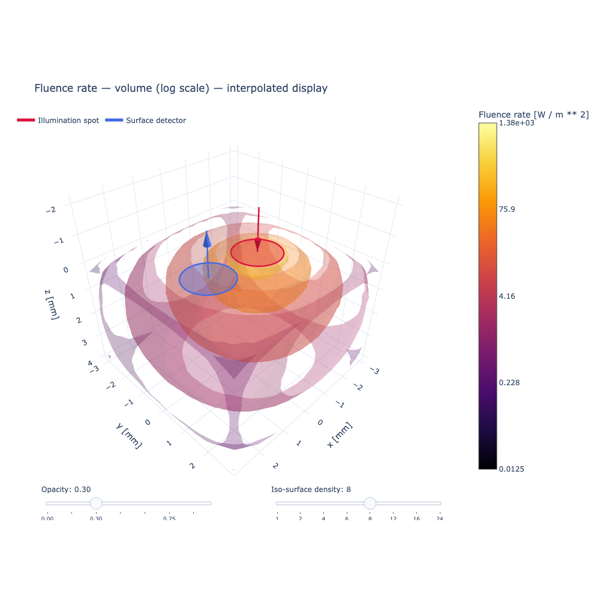
Build a layered skin sample, refine a tetrahedral mesh, and solve for fluence.
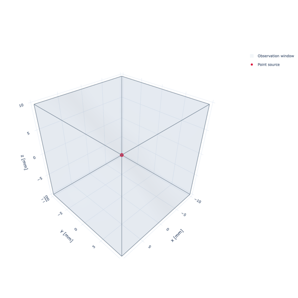
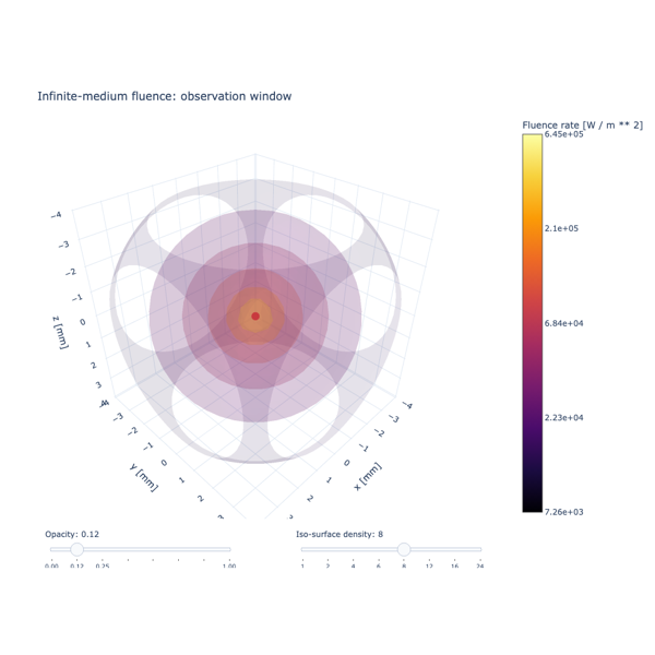
Configure a point source and observation mesh, solve the analytical P1 Green function, and explore its 3D fluence field.
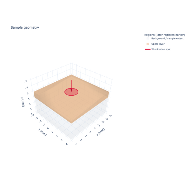
Inspect fluence, flux, and energy accounting for a finite-element solve with a disk source.
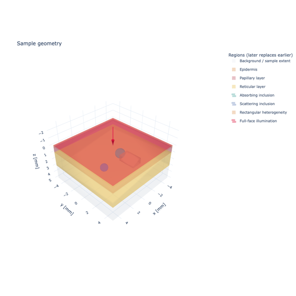
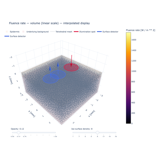
Combine layers, spheres, and a box, solve the illuminated sample, and explore its 3D fluence volume.
Samples and meshes#
Use named sample models, then create Cartesian or tetrahedral meshes.
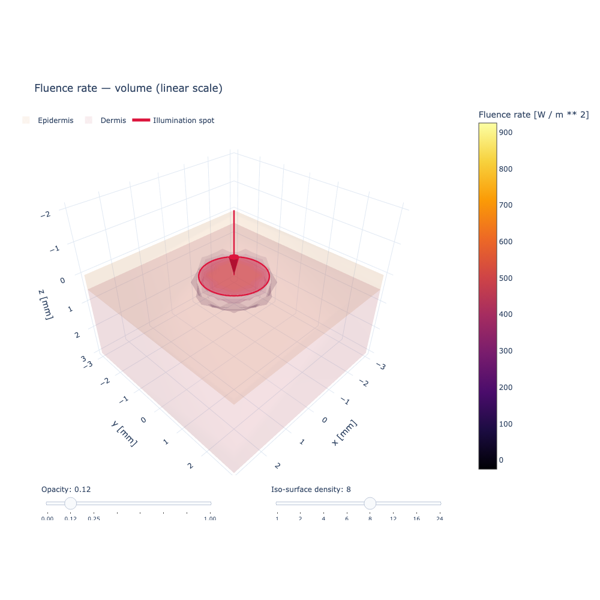
Build a two-layer skin sample and a layered phantom from explicit materials.
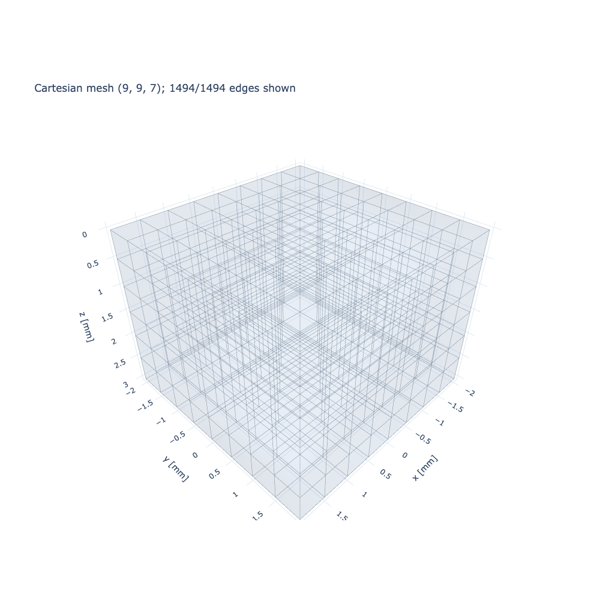
Set explicit node counts for a regular grid and plot its cell edges.
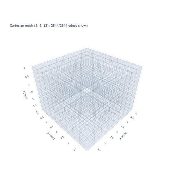
Request spacing in physical units, including anisotropic spacing by axis.
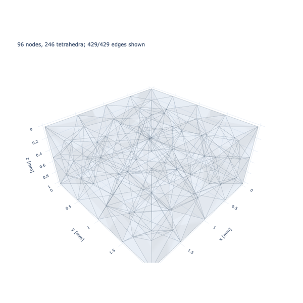
Generate and plot an unstructured tetrahedral mesh at a global target size.
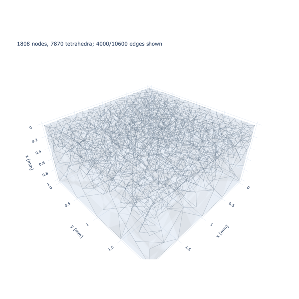
Refine a named layer and the neighborhoods around a source and detector.
Sources and detectors#
Configure diffuse illumination and contact apertures, and check detector mesh convergence.
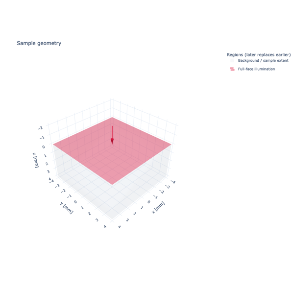
Use UniformSurfaceSource to illuminate an entire sample face and
render the resulting field in 3D.
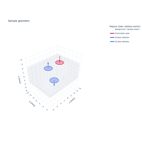
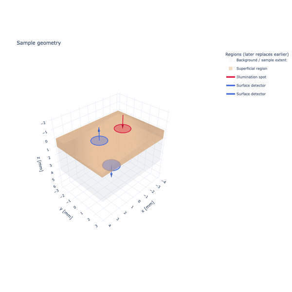
Define detector positions and acceptance cones, inspect the system, and calculate reflection and transmission signals.
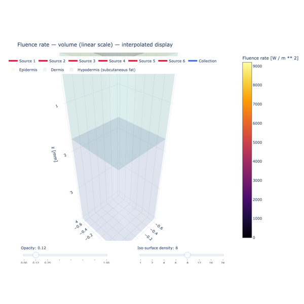
Simulate simultaneous illumination from six fibers around a central collection fiber in a layered skin model.
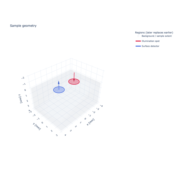
Compare detector signals and sampled source and aperture areas over successively finer meshes.
Spectral calculations#
Sweep wavelength-dependent materials and integrate source spectra and detector responsivity.
Compare Gaussian and Lorentzian wavelength profiles and attach one to a source.
Interpolate material spectra and plot collected power across wavelengths with fixed sample and instrument geometry.
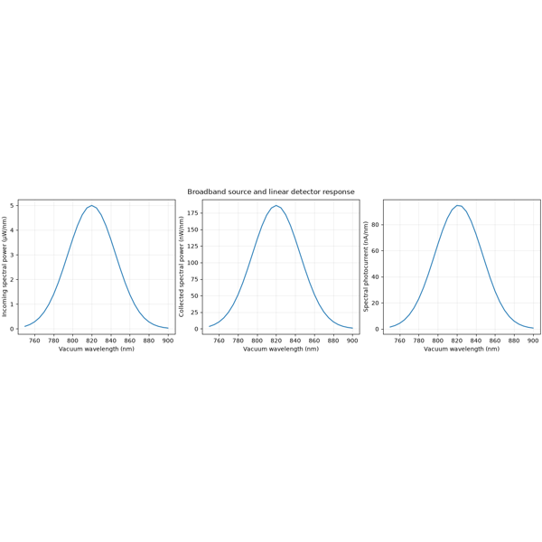
Configure the existing source with a power density and the detector with responsivity, then integrate optical power and electrical current.
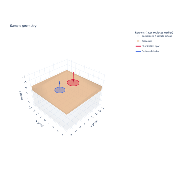
Interpolate layer-specific anisotropy and detector power across wavelengths.
Transport models#
Compare angular approximations and explore phase functions and layer anisotropy.
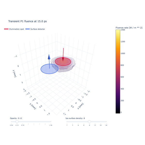
Calculate a pulsed time response and inspect the contact detector trace.
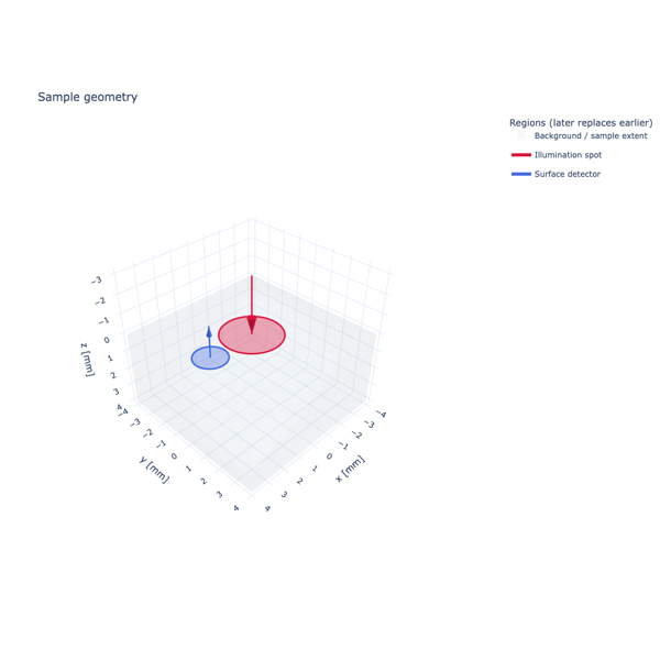
Compare detector signals from P1 and SP3 on the same sample.
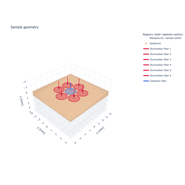
Solve the same sensor geometry with three angular approximations.
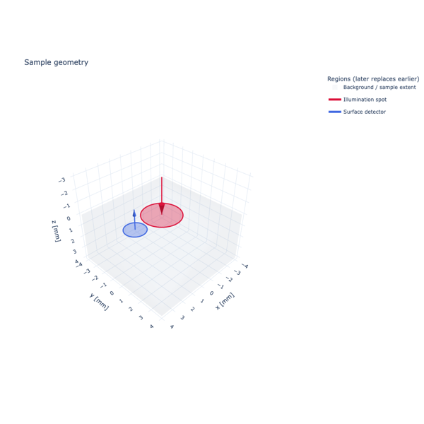
Compare phase functions with matching anisotropy but different higher moments.
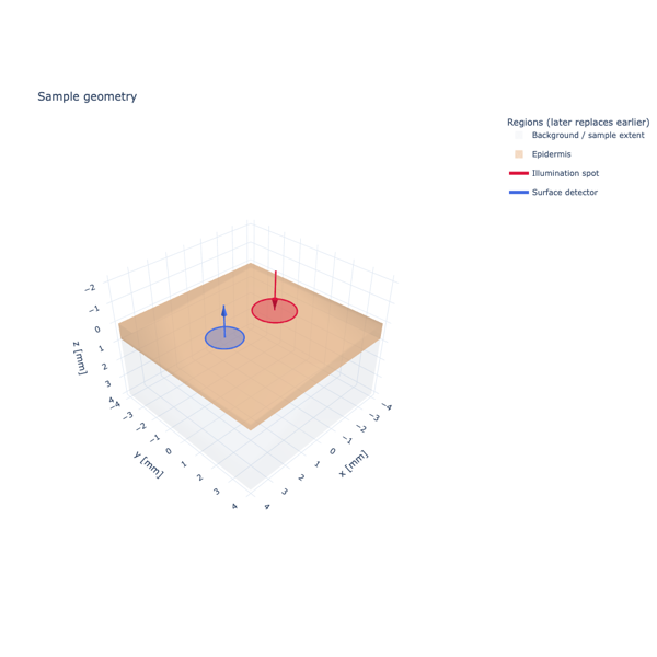
Give each material its own scattering anisotropy and solve with SP3.
Parameter studies#
Vary optical properties, fiber separation, and boundary reflectance, and examine computational scaling.
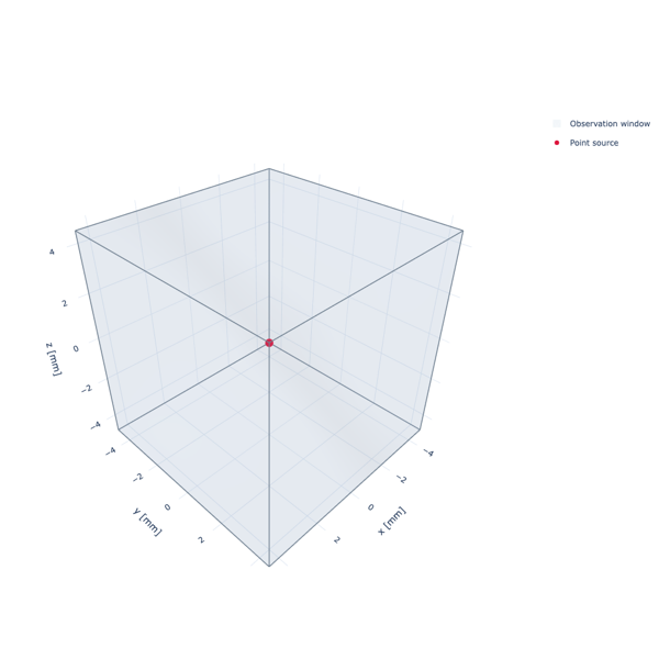
Compare fluence profiles while holding reduced scattering and source configuration fixed.
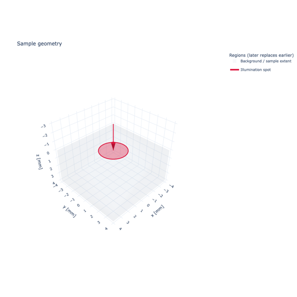
Compare centerline fluence and escaping power as diffuse reflectance changes.
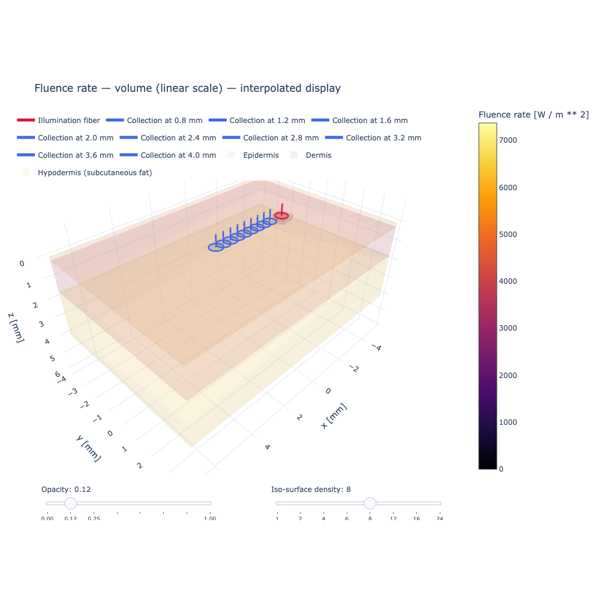
Move a collection fiber away from one illumination fiber and compare collected power as absorption increases in the middle skin layer.
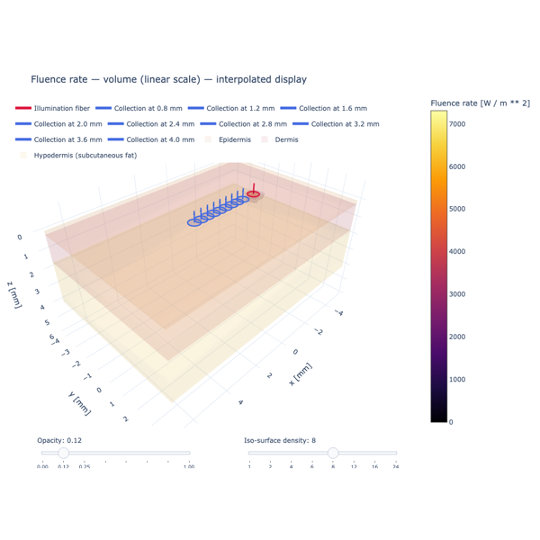
Compare equal absorption increments in epidermis, dermis, and hypodermis to explore how each layer changes the distance response.
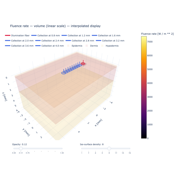
Move the dermis-hypodermis interface while keeping the outer sample and probe fixed, and compare collected power with a 1.5 mm dermis.
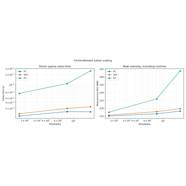
Measure solve time and peak process memory across tetrahedral mesh sizes, and use the results to decide whether iterative P3 solvers warrant study.
Validation#
Assess mesh refinement and compare calculations with independent references.
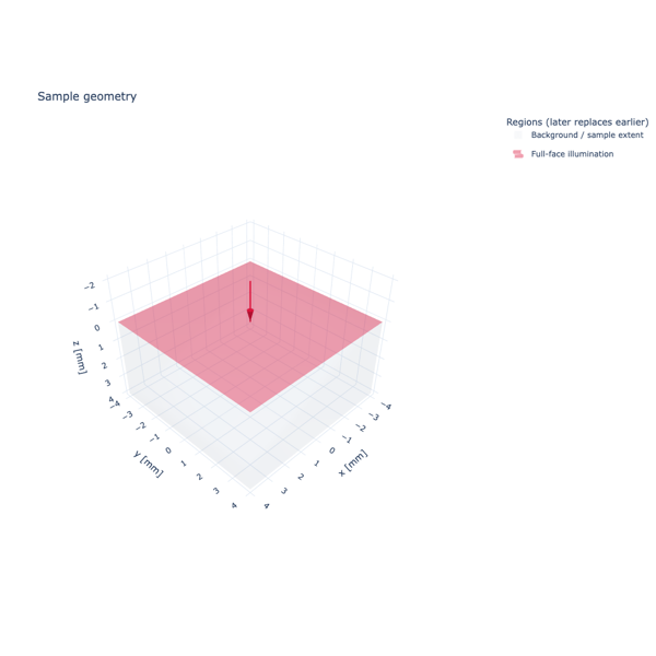
Compare fluence over three grids and inspect recorded FEM preparation, assembly, factorization, and solve timings.
Compare P1 diffusion and SP3 FEM profiles with independent closed-form and matrix-exponential slab solutions.
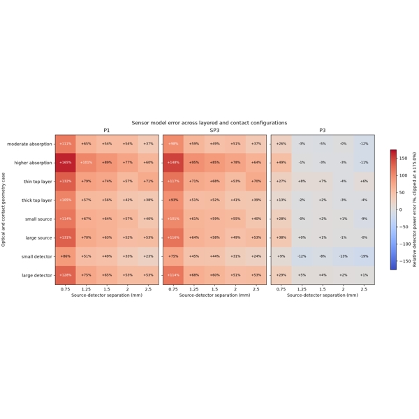
Explore published comparisons while varying layer thickness, optical properties, source size, detector radius, and source-detector separation.
Inverse problems#
Explore synthetic inverse calculations and their numerical and model limitations.
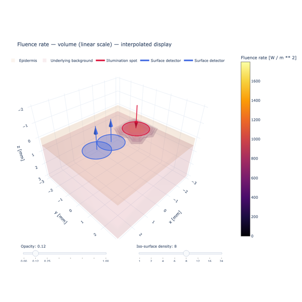
Check how refinement affects detector powers for a layered sample before attempting a synthetic fit.
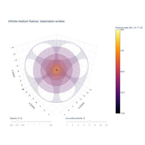
Plot the mismatch between synthetic fluence observations and candidate absorption values under the same analytical model.
Recover a model parameter from ideal simulated measurements using SciPy; the same forward model generates and fits the data.
Plotly figures embedded in the example pages are interactive: rotate, zoom, and hover to inspect the generated MomentRT data.