

Note
Go to the end to download the full example code.
Changing the diffuse boundary reflectance#
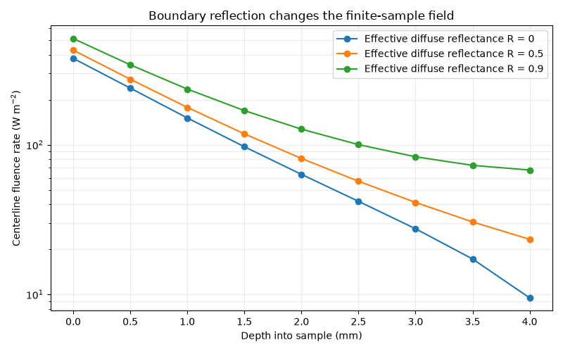
Solve the same illuminated slab with three effective diffuse reflectances. The centerline fluence increases as less diffuse current escapes through the sample boundary. The parameter is not a Fresnel reflectance. Inputs are illustrative.
import os
import matplotlib.pyplot as plt
import numpy as np
import MomentRT
from MomentRT import (
    P1,
    CartesianMesh,
    Material,
    RobinBoundary,
    Simulation,
    StructuredMedium,
    SurfaceSource,
    ureg,
)

show_figures = os.environ.get("MOMENTRT_SPHINX_GALLERY") != "1"
Define a homogeneous finite sample#
The sample is illuminated through its upper z face and uses a common refractive index throughout.
material = Material(
    phase_function=MomentRT.phase_function.HenyeyGreenstein(),
    absorption=0.03 / ureg.millimeter,
    reduced_scattering=1.0 / ureg.millimeter,
    refractive_index=1.4,
)

sample = StructuredMedium(
    origin=(-4, -4, 0) * ureg.millimeter,
    size=(8, 8, 4) * ureg.millimeter,
)

sample.add_background(
    material=material,
)

mesh = CartesianMesh.from_sample(
    sample=sample,
    shape=(13, 13, 9),
)

source = SurfaceSource(
    face="z_min",
    position=np.array([0, 0, 0]) * ureg.millimeter,
    radius=1.5 * ureg.millimeter,
    wavelength=970 * ureg.nanometer,
    optical_power=1 * ureg.milliwatt,
)
Reuse the same inputs while varying R#
Compare a more open diffuse boundary with progressively stronger internal diffuse reflection.
reflectance_values = (0.0, 0.5, 0.9)

center_index_x = mesh.shape[0] // 2

center_index_y = mesh.shape[1] // 2

depth = (
    (mesh.origin[2] + np.arange(mesh.shape[2]) * mesh.spacing[2])
    .to("millimeter")
    .magnitude
)

centerline_profiles = []

results = []

for reflectance in reflectance_values:
    boundary = RobinBoundary(
        effective_reflectance=reflectance,
    )

    solver = P1(
        boundaries=MomentRT.Boundaries.uniform(condition=boundary),
    )

    simulation = Simulation(
        medium=sample,
        source=source,
        mesh=mesh,
        solver=solver,
    )

    result = simulation.run()

    results.append(result)

    fluence = result.fluence.values.to("watt / meter**2").magnitude

    centerline_profiles.append(fluence[center_index_x, center_index_y, :])
Plot fluence through the center of the sample#
Each curve shares the same material, source power, spot, and mesh.
figure, axes = plt.subplots(figsize=(8, 5))

for reflectance, profile in zip(reflectance_values, centerline_profiles):
    axes.plot(
        depth,
        profile,
        marker="o",
        label=f"Effective diffuse reflectance R = {reflectance:g}",
    )

axes.set_yscale("log")
axes.set_xlabel("Depth into sample (mm)")
axes.set_ylabel("Centerline fluence rate (W m$^{-2}$)")
axes.set_title("Boundary reflection changes the finite-sample field")
axes.grid(True, which="both", alpha=0.25)
axes.legend()
figure.tight_layout()
Check energy accounting for each case#
The reported escape is transmitted power integrated over all sample faces.
for reflectance, result in zip(reflectance_values, results):
    incoming_power = result.energy_balance["incoming_power"].to("milliwatt")

    escaping_power = result.energy_balance["escaping_power"].to("milliwatt")

    print(
        f"R = {reflectance:g}: "
        f"incoming = {incoming_power:.4g}, "
        f"escaping = {escaping_power:.4g}"
    )

if show_figures:
    plt.show()
R = 0: incoming = 1 milliwatt, escaping = 0.838 milliwatt
R = 0.5: incoming = 1 milliwatt, escaping = 0.7425 milliwatt
R = 0.9: incoming = 1 milliwatt, escaping = 0.4101 milliwatt
Inspect the intermediate-reflectance volume#
The middle solution uses R = 0.5 and retains the same source and geometry.
volume_figure = results[1].fluence.plot(
    view="volume",
    scale="log",
    overlays=[source],
    show=show_figures,
)
Inspect the modeled geometry#
This view shows the configured geometry and instrument footprints.
gallery_system_figure = simulation.plot_system(show=False)
Total running time of the script: (0 minutes 0.406 seconds)