

Note
Go to the end to download the full example code.
Check finite-element mesh refinement#
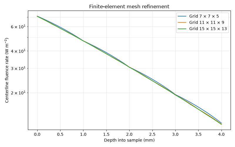
Repeat one finite-sample solve on three meshes and compare the centerline fluence profiles, then inspect a recorded P1 FEM performance benchmark. A stable curve is evidence about discretization for this setup; it does not validate the P1 approximation against radiative transfer. Sample inputs are illustrative.
import os
import matplotlib.pyplot as plt
import numpy as np
import MomentRT
from MomentRT import (
    P1,
    CartesianMesh,
    Material,
    RobinBoundary,
    Simulation,
    StructuredMedium,
    UniformSurfaceSource,
    ureg,
)

show_figures = os.environ.get("MOMENTRT_SPHINX_GALLERY") != "1"
Fix the physical sample and illumination#
Uniform surface illumination avoids adding a finite disk edge to this mesh refinement comparison.
material = Material(
    phase_function=MomentRT.phase_function.HenyeyGreenstein(),
    absorption=0.03 / ureg.millimeter,
    reduced_scattering=1.0 / ureg.millimeter,
    refractive_index=1.4,
)

sample = StructuredMedium(
    origin=(-4, -4, 0) * ureg.millimeter,
    size=(8, 8, 4) * ureg.millimeter,
)

sample.add_background(
    material=material,
)

source = UniformSurfaceSource(
    face="z_min",
    wavelength=970 * ureg.nanometer,
    optical_power=1 * ureg.milliwatt,
)

boundary = RobinBoundary(
    effective_reflectance=0.5,
)

solver = P1(
    boundaries=MomentRT.Boundaries.uniform(condition=boundary),
)
Solve on coarse, medium, and fine grids#
Each grid has nodes at the centerline and at one-millimeter depth, so those physical points can be compared directly.
mesh_shapes = (
    (7, 7, 5),
    (11, 11, 9),
    (15, 15, 13),
)

depth_profiles = []

depth_axes = []

results = []

for shape in mesh_shapes:
    mesh = CartesianMesh.from_sample(
        sample=sample,
        shape=shape,
    )

    simulation = Simulation(
        medium=sample,
        source=source,
        mesh=mesh,
        solver=solver,
    )

    result = simulation.run()

    results.append(result)

    fluence = result.fluence.values.to("watt / meter**2").magnitude

    centerline = fluence[shape[0] // 2, shape[1] // 2, :]

    depth = (
        (mesh.origin[2] + np.arange(shape[2]) * mesh.spacing[2])
        .to("millimeter")
        .magnitude
    )

    depth_profiles.append(centerline)

    depth_axes.append(depth)
Compare interpolated centerline profiles#
Interpolation puts the plotted lines on the same depth coordinates; it does not change the finite-element solution or create additional mesh resolution.
common_depth = np.linspace(0, 4, 81)

figure, axes = plt.subplots(figsize=(8, 5))

for shape, depth, profile in zip(mesh_shapes, depth_axes, depth_profiles):
    axes.plot(
        common_depth,
        np.interp(common_depth, depth, profile),
        label=f"Grid {shape[0]} × {shape[1]} × {shape[2]}",
    )

axes.set_yscale("log")
axes.set_xlabel("Depth into sample (mm)")
axes.set_ylabel("Centerline fluence rate (W m$^{-2}$)")
axes.set_title("Finite-element mesh refinement")
axes.grid(True, which="both", alpha=0.25)
axes.legend()
figure.tight_layout()
Report solver residuals and energy residuals#
Algebraic and energy residuals diagnose the solve, while profile changes show this observable’s sensitivity to mesh resolution.
Grid (7, 7, 5): linear residual = 9.366e-16, energy residual = 4.120e-18 watt
Grid (11, 11, 9): linear residual = 2.857e-15, energy residual = 1.193e-18 watt
Grid (15, 15, 13): linear residual = 6.061e-15, energy residual = -4.337e-19 watt
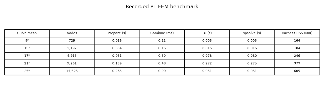
Recorded FEM timing benchmark#
The table separates geometry preparation, sparse matrix combination, LU
factorization, and the production spsolve call. It records one P1 solve
per mesh on an Apple M3 (arm64), macOS 26.6.2, Python 3.14.7, NumPy 2.5.4,
and SciPy 1.18.1. The benchmark used a homogeneous 4 mm cube with
absorption 0.02 mm⁻¹, reduced scattering 1 mm⁻¹, anisotropy 0.8, refractive
index 1.4, and effective reflectance 0.2. A 1 mW uniform source illuminated
one face at 850 nm. Preparation includes tetrahedral geometry, material
labels, element stiffness and mass assembly, boundary quadrature, and source
load. The combination column only times adding the prepared region matrices.
Assembly and factorization are medians of three repetitions; spsolve is
one wall-time measurement. Harness RSS includes the Python and SciPy runtime
and retained LU factors while another factorization is measured; it is not
the peak memory of a single production solve. Timings are machine-specific
and are not solver accuracy claims.
benchmark_rows = [
    ("9³", "729", "0.016", "0.11", "0.003", "0.003", "164"),
    ("13³", "2,197", "0.034", "0.16", "0.016", "0.016", "184"),
    ("17³", "4,913", "0.081", "0.30", "0.078", "0.080", "246"),
    ("21³", "9,261", "0.159", "0.48", "0.272", "0.275", "373"),
    ("25³", "15,625", "0.283", "0.90", "0.951", "0.951", "605"),
]

benchmark_figure, benchmark_axes = plt.subplots(figsize=(11, 3.2))

benchmark_axes.axis("off")

benchmark_table = benchmark_axes.table(
    cellText=benchmark_rows,
    colLabels=(
        "Cubic mesh",
        "Nodes",
        "Prepare (s)",
        "Combine (ms)",
        "LU (s)",
        "spsolve (s)",
        "Harness RSS (MiB)",
    ),
    cellLoc="center",
    loc="center",
)

benchmark_table.auto_set_font_size(False)

benchmark_table.set_fontsize(8)

benchmark_table.scale(1, 1.5)

benchmark_axes.set_title("Recorded P1 FEM benchmark", pad=16)

benchmark_figure.tight_layout()

if show_figures:
    plt.show()
Inspect the finest-grid fluence volume#
This view uses the final mesh from the refinement sequence. A visually smooth volume alone does not establish numerical convergence.
volume_figure = results[-1].fluence.plot(
    view="volume",
    scale="log",
    overlays=[source],
    show=show_figures,
)
Inspect the modeled geometry#
This view shows the configured geometry and instrument footprints.
gallery_system_figure = simulation.plot_system(show=False)
Total running time of the script: (0 minutes 0.539 seconds)