

Sensor-focused model validation#
Important
The data on this page use Monte Carlo reference revision 2. This corrects skipped layer interfaces and inconsistent scattering-distance sampling in the original generator. Earlier reference data distributed with versions 0.9.0 and 0.9.1 are superseded; their reported model errors must not be used to judge transport accuracy. The correction is recorded under Unreleased in the repository changelog.
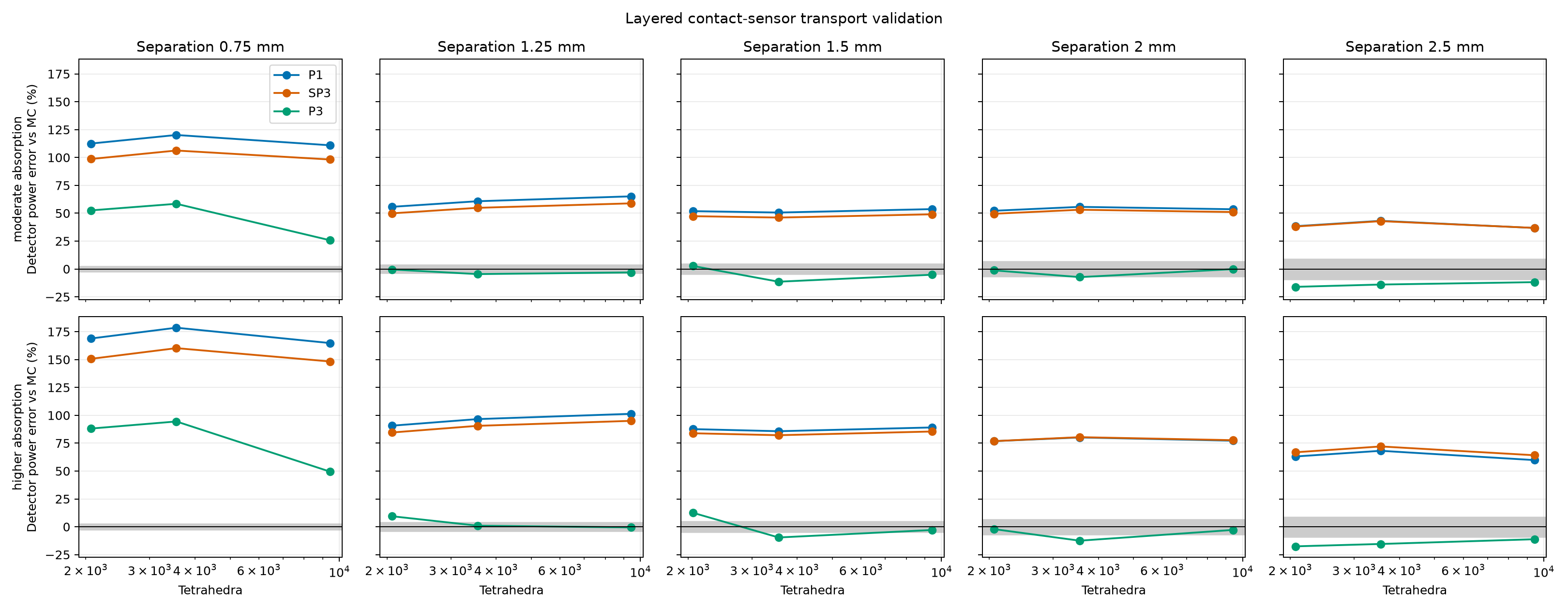
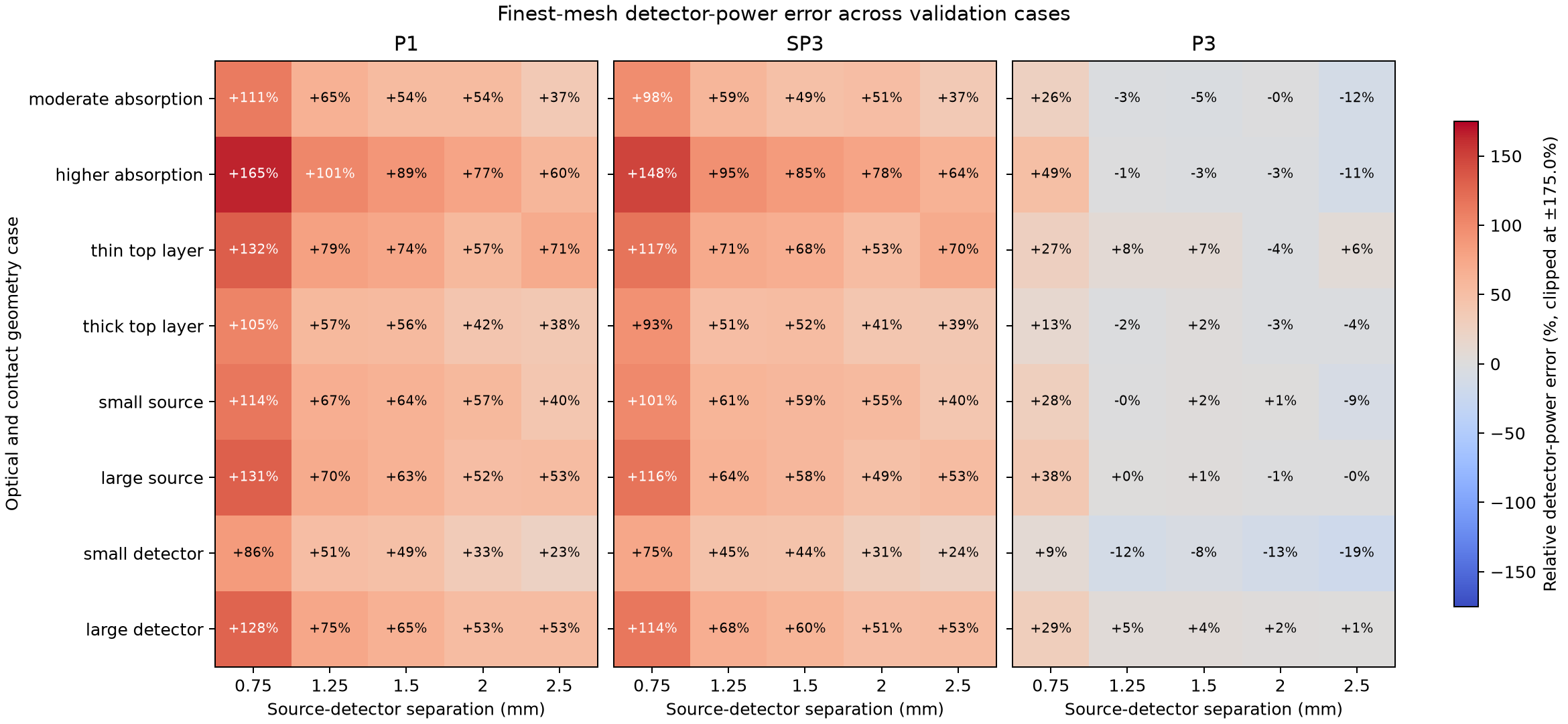
This benchmark compares P1, SP3, and P3 detector-power predictions with an independent Monte Carlo photon-transport reference across eight layered-sample and contact-sensor cases. It varies layer thickness, optical properties, source radius, detector radius, and five source-detector separations. The complete JSON report records all inputs, random seeds, detector powers, Monte Carlo standard errors, mesh sizes, sampled source and aperture areas, and runtimes. The executable gallery example visualizes these published results.
Each case uses 850 nm wavelength, 1 mW diffuse source power, 6 mm sample width,
and a 2 mm total sample thickness. The baseline layer thicknesses are
(0.25, 0.65, 1.10) mm; its source and detector radii are both 0.20 mm.
Cases vary a single geometry factor around that baseline: top-layer thickness
is changed to 0.10 or 0.45 mm, source radius to 0.10 or 0.35 mm, and detector
radius to 0.10 or 0.30 mm. For thickness variants, the bottom layer changes
to keep total sample thickness at 2 mm. A separate higher-absorption case
changes the optical coefficients in all three layers. Separations are 0.75,
1.25, 1.5, 2.0, and 2.5 mm.
The heat map compares finest-mesh detector power to Monte Carlo; colors are clipped for readability. The separate mesh-study plot shows how the baseline and higher-absorption cases change over the three mesh levels. Read both plots with the Monte Carlo uncertainty and area diagnostics in the JSON report.
The full reproducible inputs and reference data are available as
JSON.
Reproduce the benchmark from the repository root with:
.venv/bin/python tools/validate_sensor_models.py
The command writes the JSON report and both plots under
docs/source/_static/images/sensor_validation. It uses one million photon
histories per case and deterministic case-specific seeds. Use --photons
and --seed to choose another run, --cases to select named cases, or
--output-dir to write elsewhere. The committed JSON records each exact
case configuration alongside the full detector-by-detector mesh study and
sampled-area diagnostics.
Reference definition and limits#
The independent reference launches cosine-weighted diffuse photons uniformly over the source disk. It samples Henyey-Greenstein scattering using each layer’s anisotropy and converts reduced scattering to total scattering. It uses continuous absorption weighting and tallies the weighted photons that leave through each circular top-face aperture. All six sample faces transmit without Fresnel reflection, matching the benchmark’s zero-reflectance Robin boundaries. The detector accepts the full outward hemisphere, matching the Lambertian angular acceptance fraction of one used by these MomentRT detectors.
Scattering free paths are sampled with the total scattering coefficient \(\mu_s\), and absorption reduces weight by \(\exp(-\mu_a s)\) on each traveled segment. Paths stop at every layer interface, and the next segment uses that layer’s coefficients. This is the continuous absorption weighting formulation described in the MCCL documentation and by Hayakawa et al. (2014).
The reference is checked against cosine-weighted Beer-Lambert transmission through absorbing layers, exact unscattered transmission with scattering and absorption, and an independent angularly discretized RTE solution for a layered isotropically scattering slab. Further checks cover insertion of identical-material interfaces, known Henyey-Greenstein moments, and accounting for all six exit faces. These checks do not establish accuracy for every anisotropic sensor configuration or replace comparison with another mature Monte Carlo implementation. The JSON includes per-face escape, unscattered power, absorption, and energy-balance uncertainty as additional diagnostics.
These are deliberately matched boundary and detector conventions, not a complete model of an optical instrument. The reference uses independent photon histories and reports their sampling error; it does not include Fresnel reflection, a collimated LED, external optics, or detector responsivity. P1, SP3, and P3 all solve the same finite layered geometry, but their transport approximations can differ from the angularly resolved reference. Mesh refinement cannot remove model-form error. Read the plotted errors together with the Monte Carlo uncertainty and area fractions in the JSON; agreement in energy balance or sampled area alone is not evidence of transport accuracy.
The cases are illustrative and do not span the full range of tissue structures, optical properties, or sensor designs. They are a reproducible diagnostic suite, not a claim of accuracy for skin or every source-detector distance. At the finest mesh, the small-source and small-detector cases sample about 87% of their corresponding geometric footprint areas. Treat those particular results as under-resolved; refine the contact mesh before interpreting their model errors as transport-approximation error.
Explore a two-fiber absorption study#
The two-fiber skin example keeps one illumination fiber fixed and moves a collection fiber from 0.8 to 4 mm away. It compares baseline dermal absorption with 3x and 10x absorption while preserving the other layers, scattering, source power, and collection geometry. The 10x case makes the middle layer more absorbing than either adjacent layer.
In this illustrative P1 study, the 10x case retains about 76% of the baseline signal at 0.8 mm but only 1.5% at 4 mm. The largest collected-power change across the final mesh refinement is about 2.4%, and the largest sampled source/aperture area error on the finest mesh is below 1%. This supports exploring separation-dependent absorption contrast within this model; it does not establish transport accuracy or unique depth sensitivity. The example includes both meshes on the power plot and reports all three mesh levels, energy residuals, and minimum fluence, including a negative nodal value on the coarsest high-absorption mesh. Further refinement, larger-domain checks, and an independent transport reference are needed for quantitative probe design.
Two follow-on examples separate other model choices: layer-specific absorption applies the same absorption increment to one anatomical layer at a time, while dermis thickness moves the lower dermal interface at fixed optical coefficients. Both compare coarse and fine meshes across the collection-distance scan. They are forward sensitivity studies, not validated methods for identifying a tissue layer or estimating its thickness.
For the layer-specific study, adding 0.10 inverse mm to epidermis or dermis reduces the signal by about 7% at 0.8 mm in both cases. At 4 mm the reductions are about 10% and 62%, respectively; the corresponding hypodermal reduction is about 25%. The largest power change on mesh refinement is about 4.5%. These forward predictions illustrate distance-dependent contrast without establishing unique recovery of the absorbing layer.
In the thickness example, the 0.5 mm dermis gives about 2.6 times the 1.5 mm reference signal at 4 mm separation, while the 2.5 mm dermis gives about 0.77 times that signal. The largest power change between its two meshes is about 5%. The much smaller differences at 0.8 mm are not resolved well enough to support a thickness trend. These comparisons share a dermal absorption of 0.165 inverse mm and a fixed outer sample; changing thickness also replaces one scattering material with another.