

Note
Go to the end to download the full example code.
Compare sensor-validation cases#
Explore the published P1, SP3, and P3 detector-power comparisons across layer thicknesses, optical properties, source sizes, detector radii, and separations. The example reads the checked-in Monte Carlo reference report so documentation builds do not rerun the photon simulations.
import json
from pathlib import Path
import matplotlib.pyplot as plt
import numpy as np
Load the complete input and reference report#
Each case records layer thicknesses and optical properties, source and detector radii, source-detector separations, Monte Carlo standard errors, mesh sizes, sampled areas, and solver powers.
repository_root = next(
    parent
    for parent in (Path.cwd().resolve(), *Path.cwd().resolve().parents)
    if (
        parent
        / "docs"
        / "source"
        / "_static"
        / "images"
        / "sensor_validation"
        / "sensor_validation.json"
    ).is_file()
)
report_path = (
    repository_root
    / "docs"
    / "source"
    / "_static"
    / "images"
    / "sensor_validation"
    / "sensor_validation.json"
)
report = json.loads(report_path.read_text())
print(f"Monte Carlo reference revision: {report['reference_revision']}")
cases = report["cases"]
solver_names = ("P1", "SP3", "P3")
detector_offsets_mm = cases[0]["monte_carlo"]["detector_offsets_mm"]
detector_names = [f"separation_{offset:g}_mm" for offset in detector_offsets_mm]
Monte Carlo reference revision: 2
Inspect case inputs#
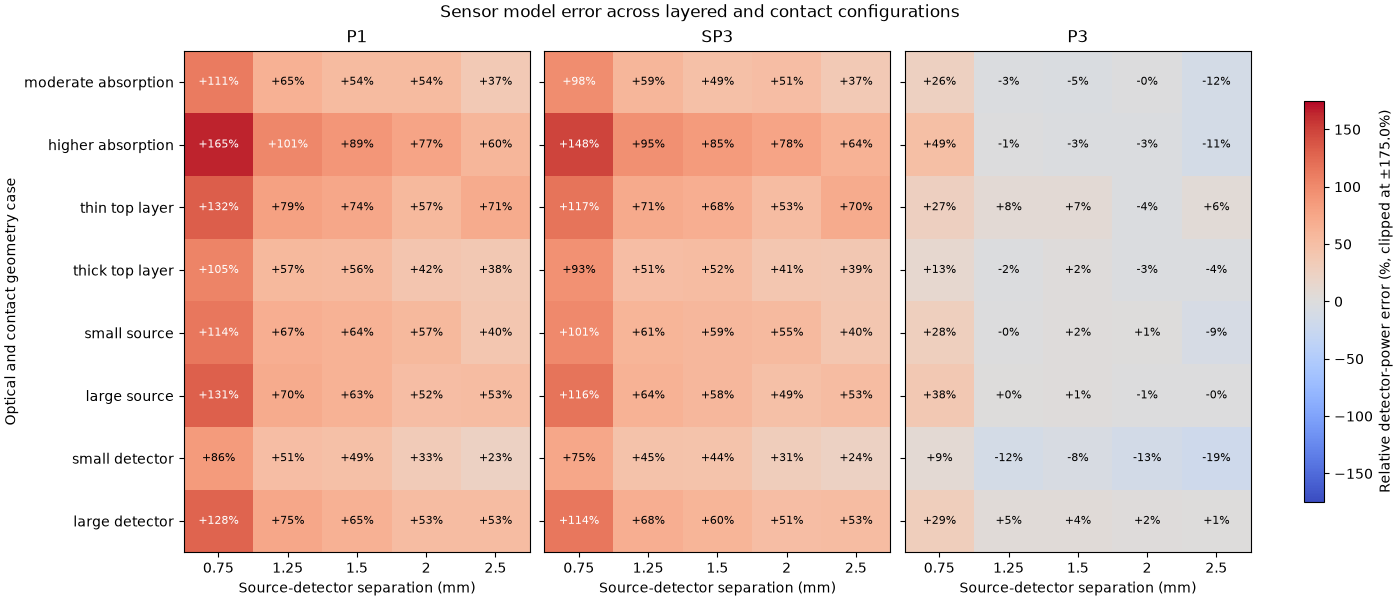
The cases vary one factor at a time around the moderate-absorption baseline, except the higher-absorption case, which changes all three layers’ optical coefficients together.
for case in cases:
    configuration = case["configuration"]
    layer_descriptions = "; ".join(
        f"{layer['thickness_mm']:g} mm: "
        f"mu_a={layer['absorption_per_mm']:g}/mm, "
        f"mu_s'={layer['reduced_scattering_per_mm']:g}/mm, "
        f"g={layer['anisotropy']:g}"
        for layer in configuration["layers"]
    )
    print(
        f"{case['name']}: source radius={configuration['source_radius_mm']:g} mm, "
        f"detector radius={configuration['detector_radius_mm']:g} mm; "
        f"{layer_descriptions}"
    )
moderate_absorption: source radius=0.2 mm, detector radius=0.2 mm; 0.25 mm: mu_a=0.18/mm, mu_s'=1.5/mm, g=0.85; 0.65 mm: mu_a=0.05/mm, mu_s'=1.1/mm, g=0.8; 1.1 mm: mu_a=0.02/mm, mu_s'=0.65/mm, g=0.75
higher_absorption: source radius=0.2 mm, detector radius=0.2 mm; 0.25 mm: mu_a=0.35/mm, mu_s'=1.2/mm, g=0.85; 0.65 mm: mu_a=0.14/mm, mu_s'=0.9/mm, g=0.8; 1.1 mm: mu_a=0.08/mm, mu_s'=0.6/mm, g=0.75
thin_top_layer: source radius=0.2 mm, detector radius=0.2 mm; 0.1 mm: mu_a=0.18/mm, mu_s'=1.5/mm, g=0.85; 0.65 mm: mu_a=0.05/mm, mu_s'=1.1/mm, g=0.8; 1.25 mm: mu_a=0.02/mm, mu_s'=0.65/mm, g=0.75
thick_top_layer: source radius=0.2 mm, detector radius=0.2 mm; 0.45 mm: mu_a=0.18/mm, mu_s'=1.5/mm, g=0.85; 0.65 mm: mu_a=0.05/mm, mu_s'=1.1/mm, g=0.8; 0.9 mm: mu_a=0.02/mm, mu_s'=0.65/mm, g=0.75
small_source: source radius=0.1 mm, detector radius=0.2 mm; 0.25 mm: mu_a=0.18/mm, mu_s'=1.5/mm, g=0.85; 0.65 mm: mu_a=0.05/mm, mu_s'=1.1/mm, g=0.8; 1.1 mm: mu_a=0.02/mm, mu_s'=0.65/mm, g=0.75
large_source: source radius=0.35 mm, detector radius=0.2 mm; 0.25 mm: mu_a=0.18/mm, mu_s'=1.5/mm, g=0.85; 0.65 mm: mu_a=0.05/mm, mu_s'=1.1/mm, g=0.8; 1.1 mm: mu_a=0.02/mm, mu_s'=0.65/mm, g=0.75
small_detector: source radius=0.2 mm, detector radius=0.1 mm; 0.25 mm: mu_a=0.18/mm, mu_s'=1.5/mm, g=0.85; 0.65 mm: mu_a=0.05/mm, mu_s'=1.1/mm, g=0.8; 1.1 mm: mu_a=0.02/mm, mu_s'=0.65/mm, g=0.75
large_detector: source radius=0.2 mm, detector radius=0.3 mm; 0.25 mm: mu_a=0.18/mm, mu_s'=1.5/mm, g=0.85; 0.65 mm: mu_a=0.05/mm, mu_s'=1.1/mm, g=0.8; 1.1 mm: mu_a=0.02/mm, mu_s'=0.65/mm, g=0.75
Compare finest-mesh detector-power errors#
Relative errors use the independent Monte Carlo detector power as the denominator. Colors are clipped at the shared scale limit for visibility; exact values and reference uncertainty remain in the JSON report.
errors = np.array(
    [
        [
            [
                case["finite_element"][solver_name][-1]["detectors"][detector_name][
                    "relative_error_percent"
                ]
                for detector_name in detector_names
            ]
            for case in cases
        ]
        for solver_name in solver_names
    ],
    dtype=float,
)
color_limit = max(100, min(200, np.ceil(np.nanmax(np.abs(errors)) / 25) * 25))
figure, axes = plt.subplots(
    1,
    len(solver_names),
    figsize=(14, max(6, 0.75 * len(cases))),
    sharey=True,
    constrained_layout=True,
)

for solver_index, (axis, solver_name) in enumerate(zip(axes, solver_names)):
    image = axis.imshow(
        np.clip(errors[solver_index], -color_limit, color_limit),
        cmap="coolwarm",
        vmin=-color_limit,
        vmax=color_limit,
        aspect="auto",
    )
    axis.set_title(solver_name)
    axis.set_xticks(
        np.arange(len(detector_offsets_mm)),
        labels=[f"{offset:g}" for offset in detector_offsets_mm],
    )
    axis.set_xlabel("Source-detector separation (mm)")
    axis.set_yticks(
        np.arange(len(cases)),
        labels=[case["name"].replace("_", " ") for case in cases],
    )
    for row in range(len(cases)):
        for column in range(len(detector_offsets_mm)):
            value = errors[solver_index, row, column]
            axis.text(
                column,
                row,
                f"{value:+.0f}%",
                ha="center",
                va="center",
                color="white" if abs(value) > color_limit * 0.55 else "black",
                fontsize=8,
            )

axes[0].set_ylabel("Optical and contact geometry case")
figure.colorbar(
    image,
    ax=axes.tolist(),
    label=f"Relative detector-power error (%, clipped at ±{color_limit}%)",
    shrink=0.8,
)
figure.suptitle("Sensor model error across layered and contact configurations")
Total running time of the script: (0 minutes 0.488 seconds)