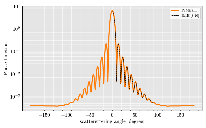
InfiniteCylinder Scatterer Bohren-Huffman figure 8.10

Importing the dependencies: numpy, matplotlib, PyMieSim

import numpy
import matplotlib.pyplot as plt
from PyMieSim.units import ureg

from PyMieSim.directories import validation_data_path
from PyMieSim.single.source import Gaussian
from PyMieSim.polarization import PolarizationState
from PyMieSim.single.scatterer import InfiniteCylinder
from PyMieSim.single import Setup

theoretical = numpy.genfromtxt(
    f"{validation_data_path}/bohren_huffman/figure_810.csv", delimiter=","
)

x = theoretical[:, 0]
y = theoretical[:, 1]

polarization_state = PolarizationState(angle=90 * ureg.degree)

source = Gaussian(
    wavelength=470 * ureg.nanometer,
    polarization=polarization_state,
    optical_power=1e-3 * ureg.watt,
    numerical_aperture=0.1,
)

scatterer = InfiniteCylinder(
    diameter=3000 * ureg.nanometer,
    material=(1.0 + 0.07j),
    medium=1.0,
)

setup = Setup(
    scatterer=scatterer,
    source=source
)

s1s2 = setup.get_representation("s1s2", sampling=800)

data = (numpy.abs(s1s2.S1) ** 2 + numpy.abs(s1s2.S2) ** 2) * (
    0.5 / (numpy.pi * source.wavenumber_vacuum.to_base_units())
) ** (1 / 4)


figure, ax = plt.subplots(1, 1)

ax.plot(s1s2.phi.to("degree").magnitude, data, "C1-", linewidth=3, label="PyMieSim")
ax.plot(x, y, "k--", linewidth=1, label="B&H [8.10]")

ax.set(
    xlabel="scattering angle [degree]",
    ylabel="Phase function",
    yscale="log",
)

ax.legend()
plt.show()


# -