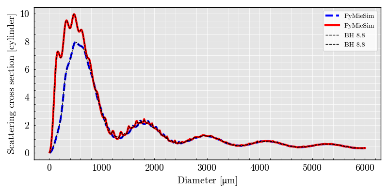
Cylinder Scatterer Bohren-Huffman figure 8.7

Importing the dependencies: numpy, matplotlib, PyMieSim

import numpy
import matplotlib.pyplot as plt
from TypedUnit import ureg

from PyMieSim.directories import validation_data_path

from PyMieSim.experiment.scatterer import Cylinder
from PyMieSim.experiment.source import Gaussian
from PyMieSim.experiment import Setup

theoretical = numpy.genfromtxt(
    f"{validation_data_path}/bohren_huffman/figure_87.csv", delimiter=","
)

diameter = numpy.geomspace(10, 6000, 800) * ureg.nanometer
volume = numpy.pi * (diameter.to_base_units().magnitude / 2) ** 2

source = Gaussian(
    wavelength=632.8 * ureg.nanometer,
    polarization=[0, 90] * ureg.degree,
    optical_power=1e-3 * ureg.watt,
    NA=0.2 * ureg.AU,
)

scatterer = Cylinder(
    diameter=diameter,
    property=1.55 * ureg.RIU,
    medium_property=1 * ureg.RIU,
    source=source,
)

experiment = Setup(
    scatterer=scatterer,
    source=source,
)

dataframe = experiment.get("Csca", add_units=False)

data = dataframe.squeeze().values.reshape([-1, diameter.size]) / volume * 1e-4 / 100

print(data.shape)

plt.figure(figsize=(8, 4))
plt.plot(diameter, data[0], "b--", linewidth=3, label="PyMieSim")
plt.plot(diameter, data[1], "r-", linewidth=3, label="PyMieSim")

plt.plot(diameter, theoretical[0], "k--", linewidth=1, label="BH 8.8")
plt.plot(diameter, theoretical[1], "k--", linewidth=1, label="BH 8.8")

plt.xlabel(r"Diameter [$\mu$m]")
plt.ylabel("Scattering cross section [cylinder]")
plt.grid(True)
plt.legend()
plt.tight_layout()
plt.show()

(2, 800)