Sphere Particles: 1

# Standard library imports
import numpy as np
import pandas as pd
import matplotlib.pyplot as plt
from TypedUnit import ureg

# PyMieSim imports
from PyMieSim.experiment.scatterer import Sphere
from PyMieSim.experiment.source import Gaussian
from PyMieSim.experiment import Setup
from PyMieSim.directories import validation_data_path
from MPSPlots.styles import mps


# Define parameters
wavelength = 632.8 * ureg.nanometer  # Wavelength of the source in meters
index = (1.4 + 0.2j) * ureg.RIU  # Refractive index of the sphere
medium_index = 1.2 * ureg.RIU  # Refractive index of the medium
optical_power = 1 * ureg.watt  # Power of the light source in watts
NA = 0.2 * ureg.AU  # Numerical aperture
diameters = (
    np.geomspace(10, 6_000, 800) * ureg.nanometer
)  # Diameters from 10 nm to 6 μm

# Configure the Gaussian source
source = Gaussian(
    wavelength=wavelength,
    polarization=0 * ureg.degree,
    optical_power=optical_power,
    NA=NA,
)

# Setup spherical scatterer
scatterer = Sphere(
    diameter=diameters, property=index, medium_property=medium_index, source=source
)

# Create experimental setup
experiment = Setup(scatterer=scatterer, source=source)

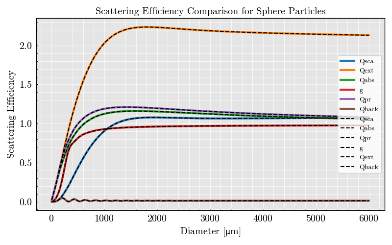
comparison_measures = ["Qsca", "Qext", "Qabs", "g", "Qpr", "Qback"]

# Compute PyMieSim scattering efficiency data
pymiesim_dataframe = experiment.get(*comparison_measures)

pymiescatt_dataframe = pd.read_csv(
    validation_data_path / "pymiescatt/example_shpere_1.csv"
)

# Plot results
with plt.style.context(mps):
    figure, ax = plt.subplots(1, 1)


pymiescatt_dataframe.diameter *= 1e9

pymiescatt_dataframe.plot(x="diameter", y=comparison_measures, ax=ax, linewidth=3)
pymiesim_dataframe.plot(
    x="scatterer:diameter",
    axes=ax,
    color="black",
    linestyle="--",
    linewidth=1.5,
    show=False,
)

ax.set(
    xlabel=r"Diameter [$\mu$m]",
    ylabel="Scattering Efficiency",
    title="Scattering Efficiency Comparison for Sphere Particles",
)
plt.legend()
plt.show()