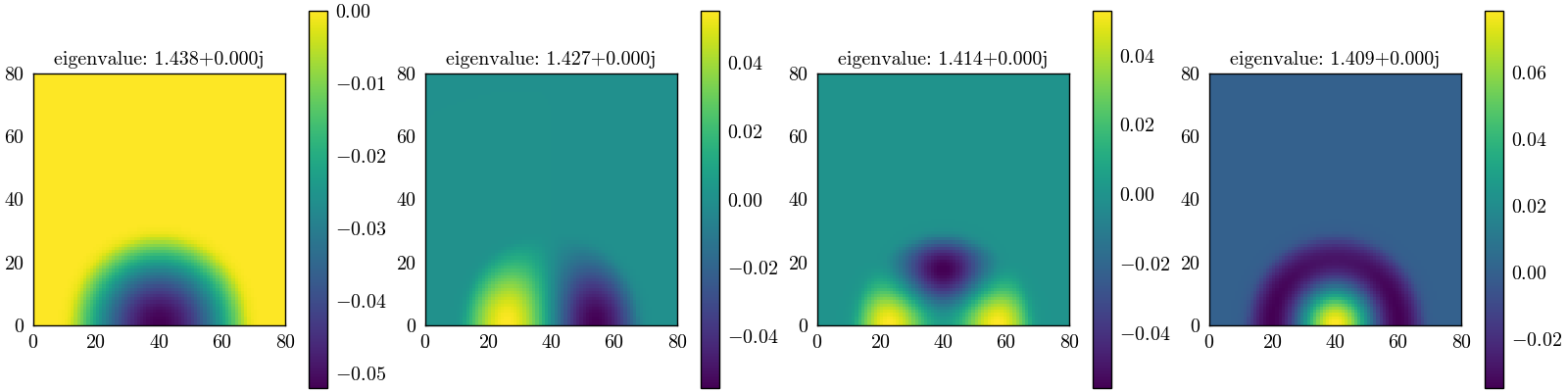
Example: 1D eigenmodes 2

In this example, we calculate and visualize the eigenmodes of a 1D finite difference operator combined with a circular mesh potential. The boundary conditions, mesh properties, and eigenmode calculations are all set up for demonstration purposes.

1D Finite-difference parameters

boundaries: {left: symmetric, right: symmetric}

derivative: 2

accuracy: 6

Importing required packages

Here we import the necessary libraries for numerical computations, rendering, and finite difference operations.

from scipy.sparse import linalg
import matplotlib.pyplot as plt
from PyFinitDiff.finite_difference_1D import FiniteDifference, get_circular_mesh_triplet, Boundaries
from PyFinitDiff import BoundaryValue

Setting up the finite difference instance and boundaries

We define the grid size and set up the finite difference instance with specified boundary conditions.

n_x = 200

sparse_instance = FiniteDifference(
    n_x=n_x,
    dx=1,
    derivative=2,
    accuracy=6,
    boundaries=Boundaries(left=BoundaryValue.SYMMETRIC, right=BoundaryValue.SYMMETRIC)
)

Creating the circular mesh potential

We create a circular mesh triplet, specifying the inner and outer values, and offset parameters.

mesh_triplet = get_circular_mesh_triplet(
    n_x=n_x,
    radius=60,
    value_out=1,
    value_in=1.4444,
    x_offset=-100
)

Combining the finite difference and mesh triplets

We add the circular mesh triplet to the finite difference operator to form the dynamic triplet.

dynamic_triplet = sparse_instance.triplet + mesh_triplet

Calculating the eigenmodes

We compute the first four eigenmodes of the combined operator using the scipy sparse linear algebra package.

eigen_values, eigen_vectors = linalg.eigs(
    dynamic_triplet.to_dense(),
    k=4,
    which='LM',
    sigma=1.4444
)

Visualizing the eigenmodes with matplotlib

We visualize the first four eigenmodes by reshaping the eigenvectors and plotting them using matplotlib.

fig, axes = plt.subplots(2, 2, figsize=(10, 8), constrained_layout=True)
axes = axes.flatten()

for i, ax in enumerate(axes):
    vector = eigen_vectors[:, i]
    ax.plot(vector)
    ax.set_title(f'eigenvalue: {eigen_values[i]:.3f}')
    ax.set_xlabel('Index')
    ax.set_ylabel('Amplitude')
    ax.grid(True)

plt.show()

/opt/hostedtoolcache/Python/3.11.13/x64/lib/python3.11/site-packages/matplotlib/cbook.py:1719: ComplexWarning: Casting complex values to real discards the imaginary part
  return math.isfinite(val)
/opt/hostedtoolcache/Python/3.11.13/x64/lib/python3.11/site-packages/matplotlib/cbook.py:1355: ComplexWarning: Casting complex values to real discards the imaginary part
  return np.asarray(x, float)