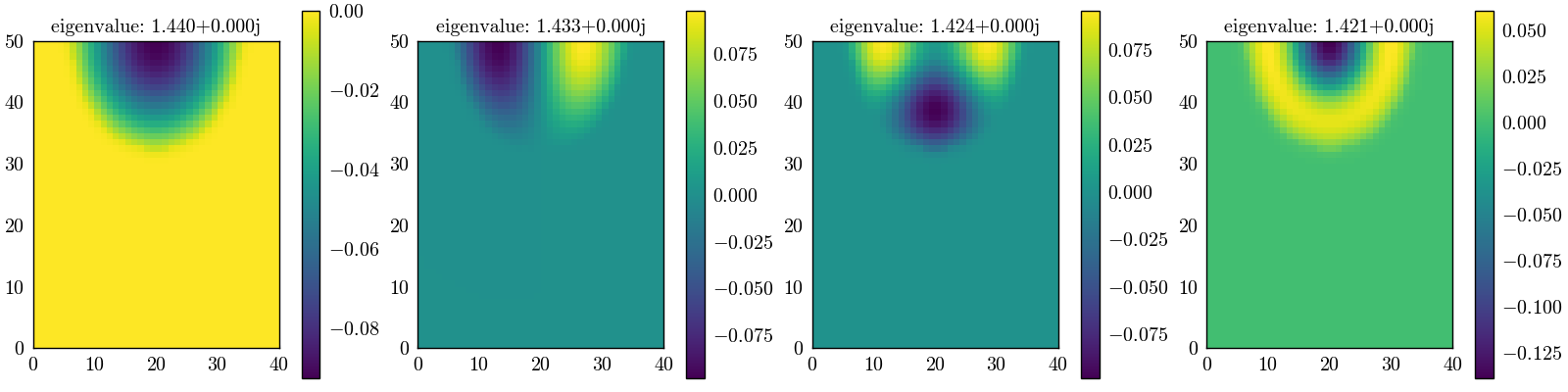
Example: eigenmodes 8

In this example, we calculate and visualize the eigenmodes of a finite difference operator combined with a circular mesh potential. The boundary conditions, mesh properties, and eigenmode calculations are all set up for demonstration purposes.

Boundaries	left	right	top	bottom
	zero	zero	sym	zero

Importing required packages

Here we import the necessary libraries for numerical computations, rendering, and finite difference operations.

from scipy.sparse import linalg
from PyFinitDiff.finite_difference_2D import FiniteDifference, get_circular_mesh_triplet, Boundaries
import matplotlib.pyplot as plt
from PyFinitDiff import BoundaryValue

Setting up the finite difference instance and boundaries

We define the grid size and set up the finite difference instance with specified boundary conditions.

n_x = 40
n_y = 50

sparse_instance = FiniteDifference(
    n_x=n_x,
    n_y=n_y,
    dx=100 / n_x,
    dy=100 / n_y,
    derivative=2,
    accuracy=2,
    boundaries=Boundaries(top=BoundaryValue.SYMMETRIC)
)

Creating the circular mesh potential

We create a circular mesh triplet, specifying the inner and outer values, and offset parameters.

mesh_triplet = get_circular_mesh_triplet(
    n_x=n_x,
    n_y=n_y,
    value_out=1.0,
    value_in=1.4444,
    x_offset=0,
    y_offset=+100,
    radius=70
)

Combining the finite difference and mesh triplets

We add the circular mesh triplet to the finite difference Laplacian to form the dynamic triplet.

dynamic_triplet = sparse_instance.triplet + mesh_triplet

Calculating the eigenmodes

We compute the first four eigenmodes of the combined operator using the scipy sparse linear algebra package.

eigen_values, eigen_vectors = linalg.eigs(
    dynamic_triplet.to_scipy_sparse(),
    k=4,
    which='LM',
    sigma=1.4444
)

shape = [sparse_instance.n_y, sparse_instance.n_x]

Visualizing the eigenmodes with matplotlib

We visualize the first four eigenmodes by reshaping the eigenvectors and plotting them using matplotlib.

fig, axes = plt.subplots(1, 4, figsize=(16, 4), constrained_layout=True)

for i, ax in enumerate(axes):
    vector = eigen_vectors[:, i].real.reshape(shape)
    mesh = ax.pcolormesh(vector, shading='auto', cmap='viridis')
    ax.set_title(f'eigenvalue: {eigen_values[i]:.3f}')
    ax.set_aspect('equal')
    plt.colorbar(mesh, ax=ax)

plt.show()