Concentration Sweep: From Isolated Events to Coincidence

This tutorial studies how increasing particle concentration changes the detector signal and the extracted event statistics. % Using the same optical, electronic, and digital processing configuration, we run a series of simulations at progressively higher concentrations and compare the resulting analog traces, trigger counts, and peak distributions.

Questions addressed

1. When do individual particle pulses begin to overlap?

2. How does concentration affect the number of detected events?

3. How do peak height and area distributions change as coincidence increases?

4. When does the measured signal cease to reflect single-particle behavior?

from FlowCyPy.units import ureg
from FlowCyPy import FlowCytometer
from FlowCyPy.fluidics import (
    Fluidics,
    FlowCell,
    ScattererCollection,
    populations,
    distributions,
    SampleFlowRate,
    SheathFlowRate,
)
from FlowCyPy.opto_electronics import (
    Detector,
    Digitizer,
    OptoElectronics,
    Amplifier,
    circuits,
    source,
)
from FlowCyPy.digital_processing import (
    DigitalProcessing,
    discriminator,
    peak_locator,
)

Step 1: Build a reusable cytometer configuration

flow_cell = FlowCell(
    sample_volume_flow=SampleFlowRate.MEDIUM.value,
    sheath_volume_flow=SheathFlowRate.MEDIUM.value,
    width=400 * ureg.micrometer,
    height=150 * ureg.micrometer,
)

excitation_source = source.Gaussian(
    waist_z=10e-6 * ureg.meter,
    waist_y=60e-6 * ureg.meter,
    wavelength=405 * ureg.nanometer,
    optical_power=100 * ureg.milliwatt,
    rin=-140 * ureg.dB_per_Hz,
    bandwidth=10 * ureg.megahertz,
)

detectors = [
    Detector(
        name="side",
        phi_angle=90 * ureg.degree,
        numerical_aperture=1.1,
        responsivity=1 * ureg.ampere / ureg.watt,
    )
]

amplifier = Amplifier(
    gain=10 * ureg.volt / ureg.ampere,
    bandwidth=10 * ureg.megahertz,
    voltage_noise_density=0.0 * ureg.nanovolt / ureg.sqrt_hertz,
    current_noise_density=0.0 * ureg.femtoampere / ureg.sqrt_hertz,
)

digitizer = Digitizer(
    sampling_rate=60 * ureg.megahertz,
    bit_depth=14,
    use_auto_range=True,
    channel_range_mode="shared",
)


analog_processing = [
    circuits.BaselineRestorationServo(time_constant=100 * ureg.microsecond),
    circuits.BesselLowPass(cutoff_frequency=2 * ureg.megahertz, order=4, gain=2),
]

opto_electronics = OptoElectronics(
    digitizer=digitizer,
    detectors=detectors,
    source=excitation_source,
    analog_processing=analog_processing,
    amplifier=amplifier,
)

digital_processing = DigitalProcessing(
    discriminator=discriminator.DynamicWindow(
        trigger_channel="side",
        threshold="4sigma",
        pre_buffer=30,
        post_buffer=30,
        max_triggers=-1,
    ),
    peak_algorithm=peak_locator.GlobalPeakLocator(),
)

Step 2: Sweep concentration

medium_refractive_index = distributions.Delta(1.33)
diameter_distribution = distributions.RosinRammler(
    scale=120 * ureg.nanometer,
    shape=8,
)
refractive_index_distribution = distributions.Normal(
    mean=1.44,
    standard_deviation=0.002,
    low_cutoff=1.33,
)

concentration_values = [
    1e8,
    5e8,
    1e9,
    5e9,
]

run_records = []

for concentration_value in concentration_values:
    scatterer_collection = ScattererCollection()

    population = populations.SpherePopulation(
        name=f"{concentration_value:.0e} particles_per_mL",
        medium_refractive_index=medium_refractive_index,
        concentration=concentration_value * ureg.particle / ureg.milliliter,
        diameter=diameter_distribution,
        refractive_index=refractive_index_distribution,
        sampling_method=populations.ExplicitModel(),
    )

    scatterer_collection.add_population(population)

    fluidics = Fluidics(
        scatterer_collection=scatterer_collection,
        flow_cell=flow_cell,
    )

    cytometer = FlowCytometer(
        fluidics=fluidics,
        background_power=0.001 * ureg.milliwatt,
    )

    run_record = cytometer.run(
        opto_electronics=opto_electronics,
        digital_processing=digital_processing,
        run_time=1 * ureg.millisecond,
    )

    run_records.append(run_record)

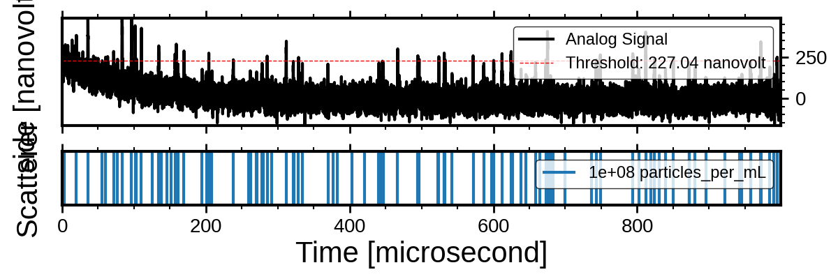
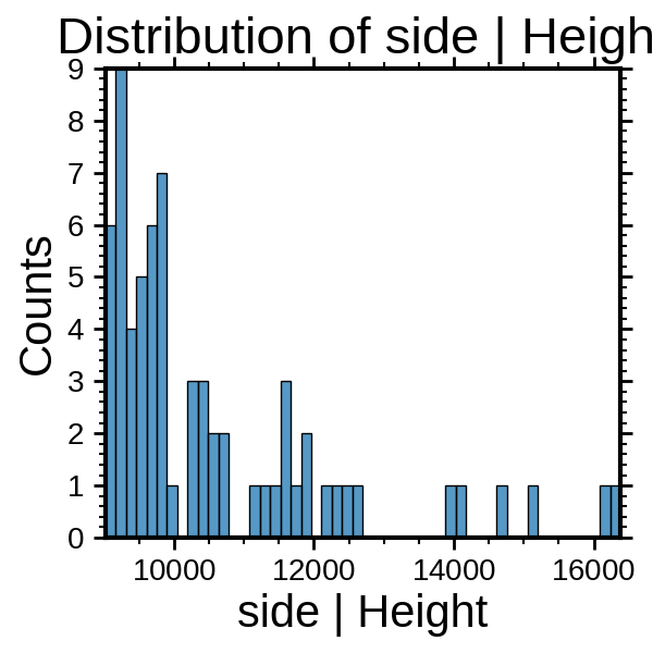
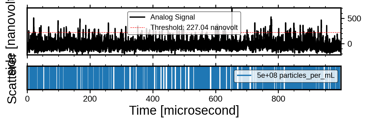
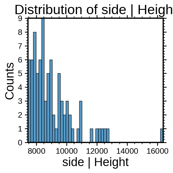
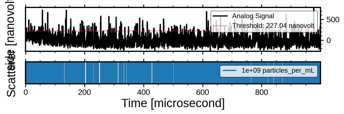
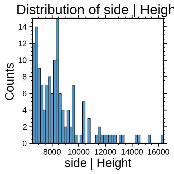
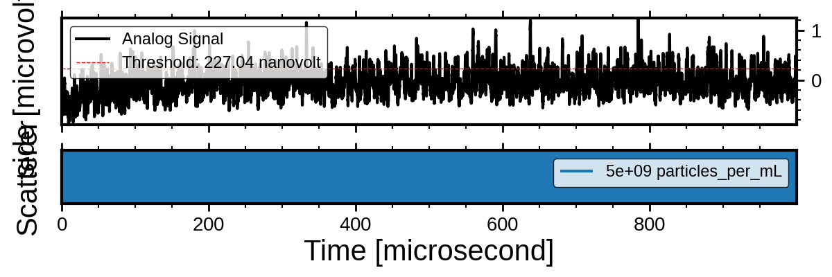
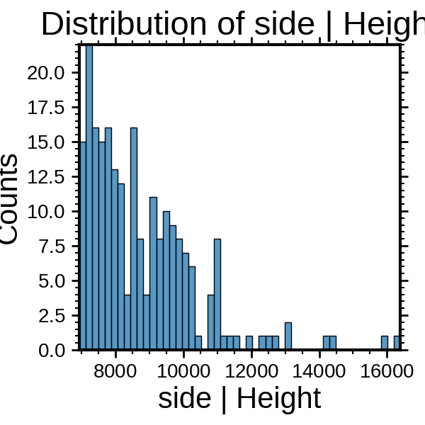
Step 3: Compare analog traces and extracted events

for run_record in run_records:
    _ = run_record.plot_analog(figure_size=(12, 4))
    _ = run_record.plot_peaks(x=("side", "Height"))

• 
• 
• 
• 
• 
• 
• 
•