Flow Cytometry Simulation: Full System Example with Workflow

This tutorial demonstrates a complete flow cytometry simulation using the FlowCyPy library. It models fluidics, optics, signal processing, and classification of multiple particle populations.

Steps Covered:

1. Configure simulation parameters and noise models

2. Define laser source, flow cell geometry, and fluidics

3. Add synthetic particle populations

4. Set up detectors, amplifier, and digitizer

5. Simulate analog and digital signal acquisition

6. Apply triggering and peak detection

7. Classify particle events based on peak features

from FlowCyPy.workflow import (
    ureg,
    SimulationSettings,
    Workflow,
    Detector,
    circuits,
    peak_locator,
    triggering_system,
    distributions,
    population,
    GammaModel,
    classifiers,
)

SimulationSettings.include_noises = False
SimulationSettings.include_shot_noise = True
SimulationSettings.include_dark_current_noise = True
SimulationSettings.include_source_noise = True
SimulationSettings.include_amplifier_noise = True
SimulationSettings.assume_perfect_hydrodynamic_focusing = True
SimulationSettings.population_cutoff_bypass = False

population_0 = population.Sphere(
    name="Pop 0",
    medium_refractive_index=distributions.Delta(1.33 * ureg.RIU),
    concentration=5e10 * ureg.particle / ureg.milliliter,
    diameter=distributions.RosinRammler(
        shape=150 * ureg.nanometer,
        scale=50 * ureg.nanometer,
        low_cutoff=50.0 * ureg.nanometer,
    ),
    refractive_index=distributions.Normal(
        mean=1.44 * ureg.RIU,
        standard_deviation=0.002 * ureg.RIU,
        low_cutoff=1.33 * ureg.RIU,
    ),
)

population_1 = population.Sphere(
    name="Pop 1",
    medium_refractive_index=distributions.Delta(1.33 * ureg.RIU),
    concentration=5e17 * ureg.particle / ureg.milliliter,
    diameter=distributions.RosinRammler(
        shape=50 * ureg.nanometer,
        scale=50 * ureg.nanometer,
    ),
    refractive_index=distributions.Normal(
        mean=1.44 * ureg.RIU,
        standard_deviation=0.002 * ureg.RIU,
        low_cutoff=1.33 * ureg.RIU,
    ),
    sampling_method=GammaModel(mc_samples=10_000),
)


detector_0 = Detector(
    name="side",
    phi_angle=90 * ureg.degree,
    numerical_aperture=0.3 * ureg.AU,
    responsivity=1 * ureg.ampere / ureg.watt,
)

detector_1 = Detector(
    name="forward",
    phi_angle=0 * ureg.degree,
    numerical_aperture=0.3 * ureg.AU,
    responsivity=1 * ureg.ampere / ureg.watt,
)

discriminator = triggering_system.DynamicWindow(
    trigger_detector_name="forward",
    threshold="2sigma",
    pre_buffer=20,
    post_buffer=20,
)

peak_locator = peak_locator.GlobalPeakLocator(compute_width=False)

analog_processing = [
    circuits.BaselineRestorator(window_size=10 * ureg.microsecond),
    circuits.BesselLowPass(cutoff=2 * ureg.megahertz, order=4, gain=2),
]

workflow = Workflow(
    wavelength=405 * ureg.nanometer,
    source_numerical_aperture=0.1 * ureg.AU,
    optical_power=200 * ureg.milliwatt,
    sample_volume_flow=80 * ureg.microliter / ureg.minute,
    sheath_volume_flow=1 * ureg.milliliter / ureg.minute,
    width=200 * ureg.micrometer,
    height=100 * ureg.micrometer,
    populations=[population_0, population_1],
    gain=10 * ureg.volt / ureg.ampere,
    bandwidth=10 * ureg.megahertz,
    bit_depth="14bit",
    sampling_rate=60 * ureg.megahertz,
    saturation_levels="auto",
    background_power=0.001 * ureg.milliwatt,
    detectors=[detector_0, detector_1],
    analog_processing=analog_processing,
    trigger=discriminator,
    peak_locator=peak_locator,
)

workflow.initialize()

run_record = workflow.run(run_time=1 * ureg.millisecond)

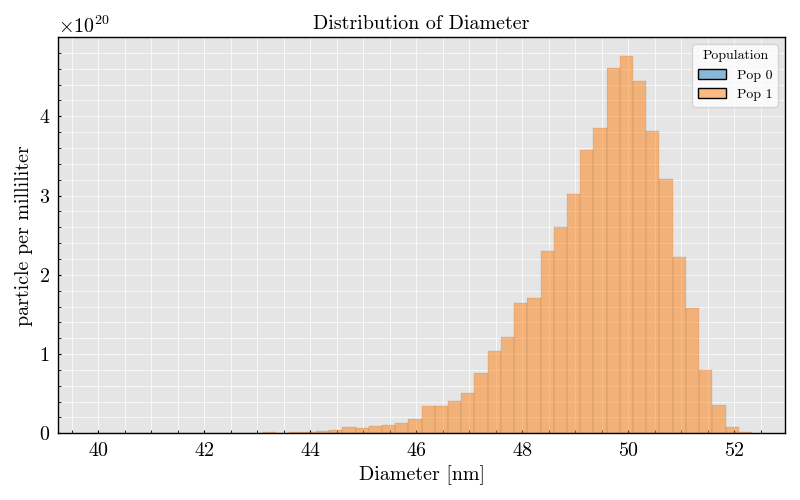
_ = run_record.event_collection.plot(x="Diameter")

Step 5: Plot Events and Raw Analog Signals

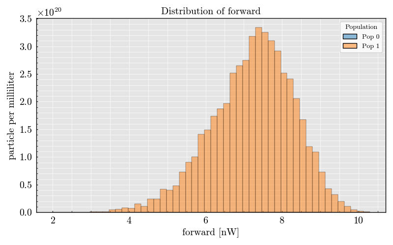
_ = run_record.event_collection.plot(x="forward")

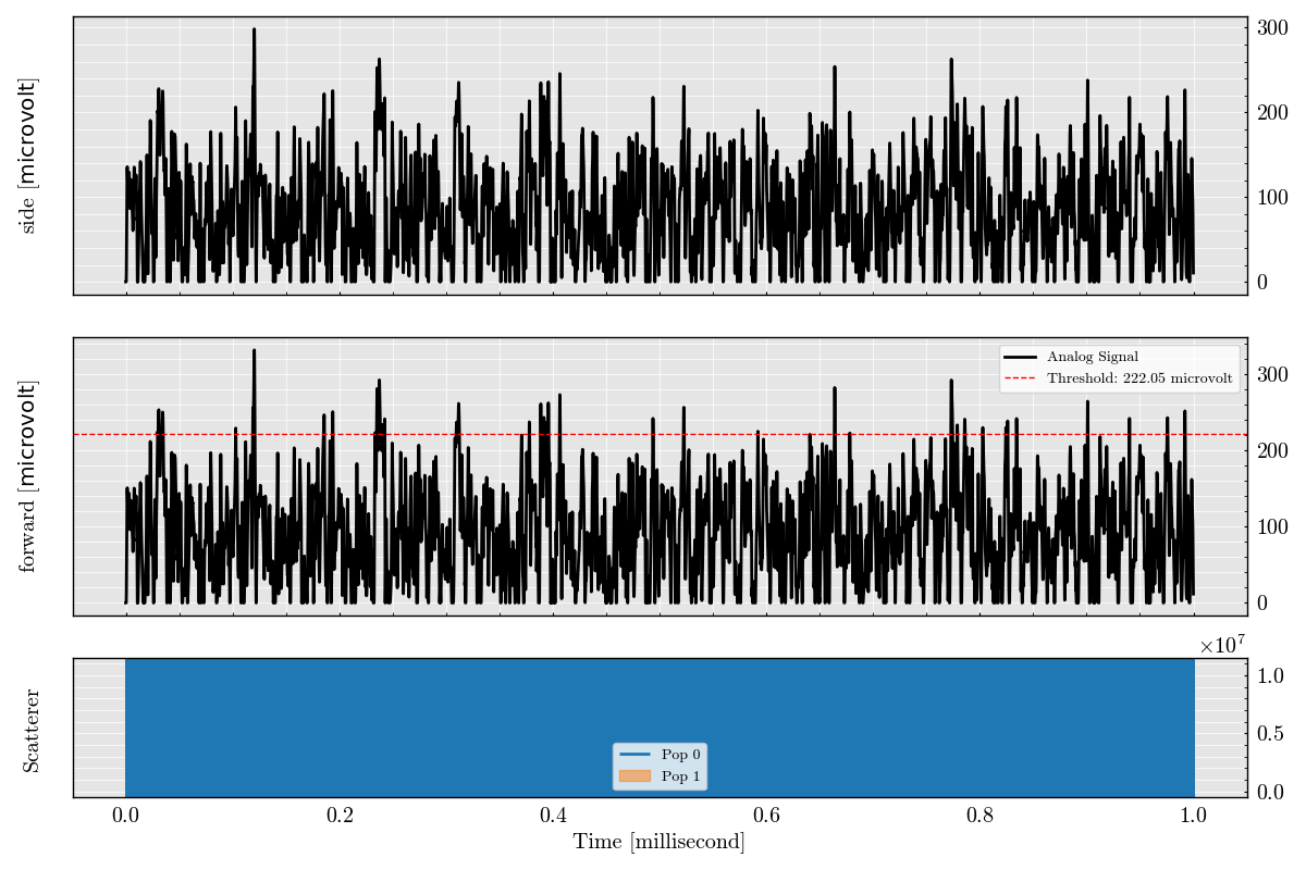
Plot raw analog signals

_ = run_record.plot_analog(figure_size=(12, 8))

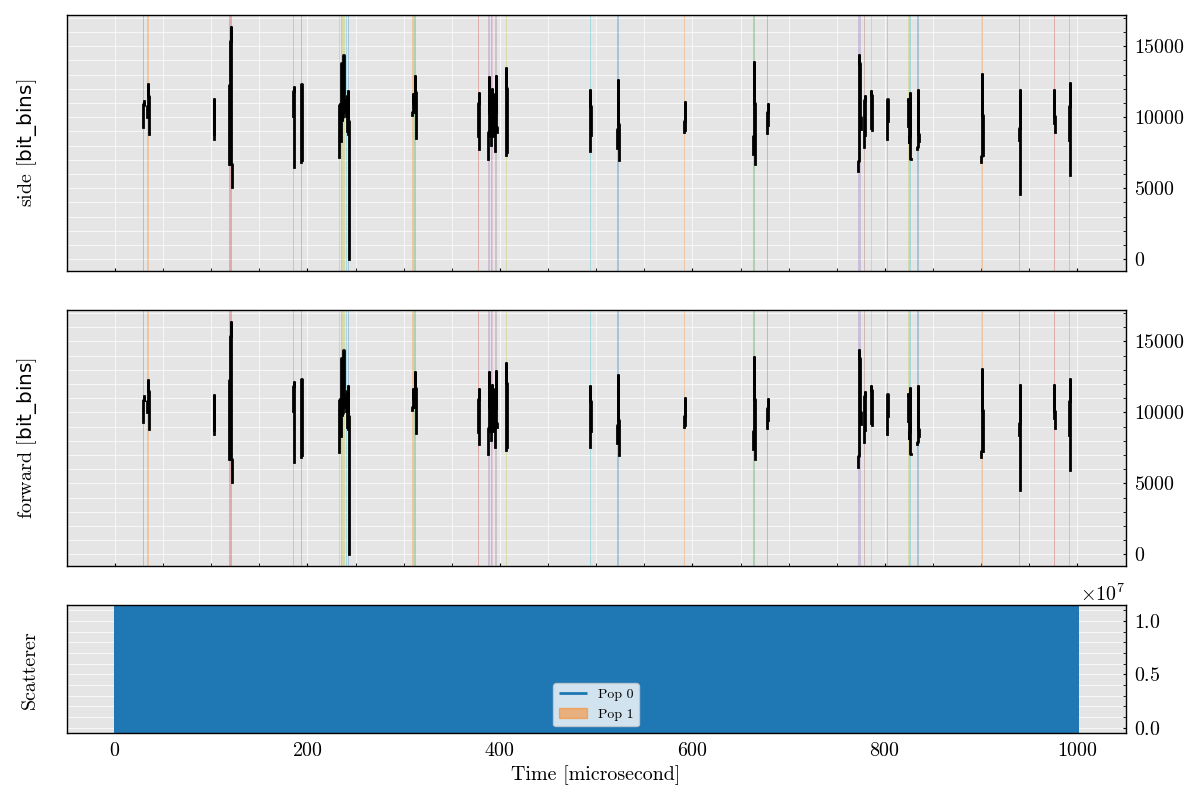
Step 6: Plot Triggered Analog Segments

_ = run_record.plot_digital(figure_size=(12, 8))

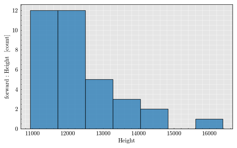
Step 7: Plot Peak Features

_ = run_record.peaks.plot(x=("forward", "Height"))

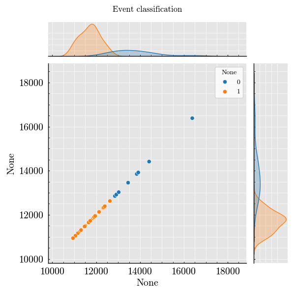
Step 8: Classify Events from Peak Features

classifier = classifiers.KmeansClassifier(number_of_clusters=2)

classified = classifier.run(
    dataframe=run_record.peaks.unstack("Detector"),
    features=["Height"],
    detectors=["side", "forward"],
)

_ = classified.plot(x=("side", "Height"), y=("forward", "Height"))