Flow Cytometry Simulation: Full System Example

This tutorial demonstrates a complete flow cytometry simulation using the FlowCyPy library. It models fluidics, optics, signal processing, and classification of multiple particle populations.

Steps Covered:

1. Configure simulation parameters and noise models

2. Define laser source, flow cell geometry, and fluidics

3. Add synthetic particle populations

4. Set up detectors, amplifier, and digitizer

5. Simulate analog and digital signal acquisition

6. Apply triggering and peak detection

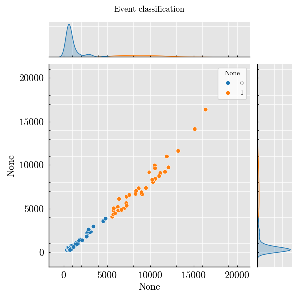
7. Classify particle events based on peak features

Step 0: Global Settings and Imports

from TypedUnit import ureg

from FlowCyPy import SimulationSettings

SimulationSettings.include_noises = False
SimulationSettings.include_shot_noise = True
SimulationSettings.include_dark_current_noise = True
SimulationSettings.include_source_noise = True
SimulationSettings.include_amplifier_noise = True
SimulationSettings.assume_perfect_hydrodynamic_focusing = True
SimulationSettings.population_cutoff_bypass = False

Step 1: Define Flow Cell and Fluidics

from FlowCyPy.fluidics import FlowCell
from FlowCyPy.fluidics import Fluidics, ScattererCollection, populations

# from FlowCyPy.sampling_method import GammaModel, ExplicitModel
from FlowCyPy.fluidics import distributions

flow_cell = FlowCell(
    sample_volume_flow=80 * ureg.microliter / ureg.minute,
    sheath_volume_flow=1 * ureg.milliliter / ureg.minute,
    width=200 * ureg.micrometer,
    height=100 * ureg.micrometer,
)

scatterer_collection = ScattererCollection()

medium_refractive_index = distributions.Delta(1.33 * ureg.RIU)

diameter_dist = distributions.RosinRammler(
    scale=50 * ureg.nanometer,
    shape=150,
    low_cutoff=50.0 * ureg.nanometer,
)


ri_dist = distributions.Normal(
    mean=1.44 * ureg.RIU,
    standard_deviation=0.002 * ureg.RIU,
    low_cutoff=1.33 * ureg.RIU,
)

sampling_method = populations.ExplicitModel()

population_0 = populations.SpherePopulation(
    name="Pop 0",
    medium_refractive_index=medium_refractive_index,
    concentration=5e10 * ureg.particle / ureg.milliliter,
    diameter=diameter_dist,
    refractive_index=ri_dist,
    sampling_method=sampling_method,
)


diameter_dist = distributions.RosinRammler(
    scale=50 * ureg.nanometer,
    shape=50,
)

ri_dist = distributions.Normal(
    mean=1.44 * ureg.RIU,
    standard_deviation=0.002 * ureg.RIU,
    low_cutoff=1.33 * ureg.RIU,
)

sampling_method = populations.GammaModel(number_of_samples=10_000)

population_1 = populations.SpherePopulation(
    name="Pop 1",
    medium_refractive_index=medium_refractive_index,
    concentration=5e17 * ureg.particle / ureg.milliliter,
    diameter=diameter_dist,
    refractive_index=ri_dist,
    sampling_method=sampling_method,
)

scatterer_collection.add_population(population_0)

scatterer_collection.dilute(factor=280)

fluidics = Fluidics(scatterer_collection=scatterer_collection, flow_cell=flow_cell)

Step 2: Define Optical Subsystem

from FlowCyPy.opto_electronics import (
    Detector,
    OptoElectronics,
    TransimpedanceAmplifier,
    source,
)

source = source.GaussianBeam(
    numerical_aperture=0.1 * ureg.AU,
    wavelength=405 * ureg.nanometer,
    optical_power=200 * ureg.milliwatt,
    RIN=-180,
)

detectors = [
    Detector(
        name="side",
        phi_angle=90 * ureg.degree,
        numerical_aperture=0.3 * ureg.AU,
        responsivity=1 * ureg.ampere / ureg.watt,
    ),
    Detector(
        name="forward",
        phi_angle=0 * ureg.degree,
        numerical_aperture=0.3 * ureg.AU,
        responsivity=1 * ureg.ampere / ureg.watt,
    ),
]

amplifier = TransimpedanceAmplifier(
    gain=10 * ureg.volt / ureg.ampere,
    bandwidth=10 * ureg.megahertz,
    voltage_noise_density=0.1 * ureg.nanovolt / ureg.sqrt_hertz,
    current_noise_density=0.2 * ureg.femtoampere / ureg.sqrt_hertz,
)

opto_electronics = OptoElectronics(
    detectors=detectors, source=source, amplifier=amplifier
)

Step 3: Signal Processing Configuration

from FlowCyPy.signal_processing import (
    Digitizer,
    SignalProcessing,
    circuits,
    peak_locator,
    triggering_system,
)

digitizer = Digitizer(
    bit_depth="14bit", saturation_levels="auto", sampling_rate=60 * ureg.megahertz
)

analog_processing = [
    circuits.BaselineRestorator(window_size=10 * ureg.microsecond),
    circuits.BesselLowPass(cutoff=2 * ureg.megahertz, order=4, gain=2),
]

triggering = triggering_system.DynamicWindow(
    trigger_detector_name="forward",
    threshold="4sigma",
    pre_buffer=20,
    post_buffer=20,
    max_triggers=-1,
)

peak_algo = peak_locator.GlobalPeakLocator(compute_width=False)

signal_processing = SignalProcessing(
    digitizer=digitizer,
    analog_processing=analog_processing,
    triggering_system=triggering,
    peak_algorithm=peak_algo,
)

Step 4: Run Simulation

from FlowCyPy import FlowCytometer

cytometer = FlowCytometer(
    opto_electronics=opto_electronics,
    fluidics=fluidics,
    signal_processing=signal_processing,
    background_power=0.001 * ureg.milliwatt,
)

run_record = cytometer.run(run_time=3 * ureg.millisecond)

_ = run_record.event_collection.plot(x="Diameter")

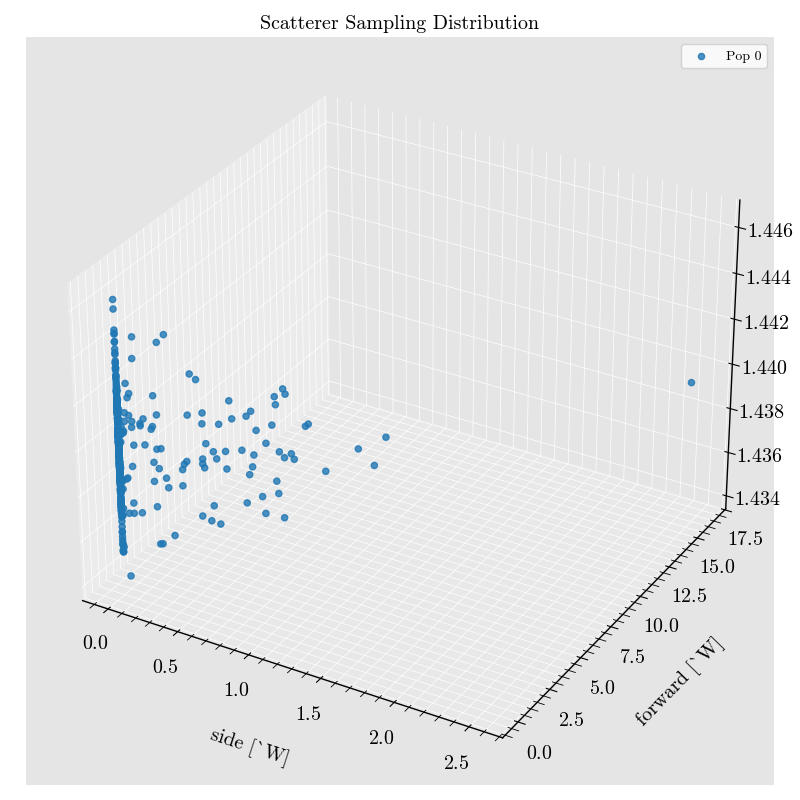
Step 5: Plot Events and Raw Analog Signals

_ = run_record.event_collection.plot(x="forward")

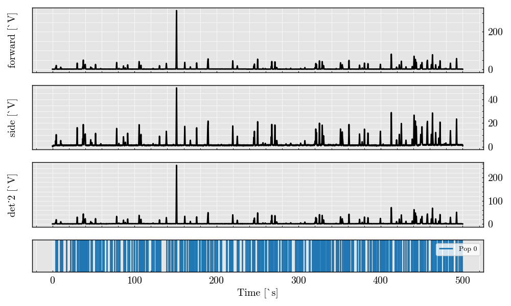
Plot raw analog signals

_ = run_record.plot_analog(figure_size=(12, 8))

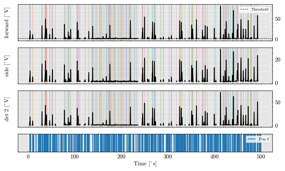
Step 6: Plot Triggered Analog Segments

_ = run_record.plot_digital(figure_size=(12, 8))

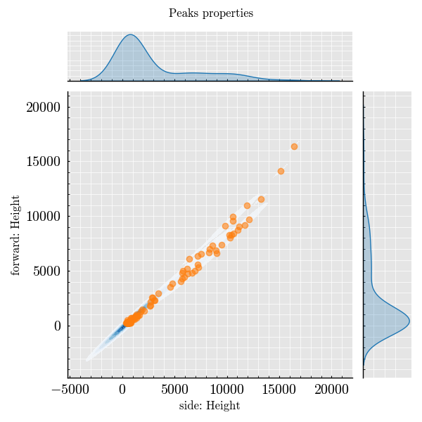
Step 7: Plot Peak Features

_ = run_record.peaks.plot(x=("forward", "Height"))

Step 8: Classify Events from Peak Features

from FlowCyPy.classifier import KmeansClassifier

classifier = KmeansClassifier(number_of_clusters=2)

classified = classifier.run(
    dataframe=run_record.peaks.unstack("Detector"),
    features=["Height"],
    detectors=["side", "forward"],
)

_ = classified.plot(x=("side", "Height"), y=("forward", "Height"))