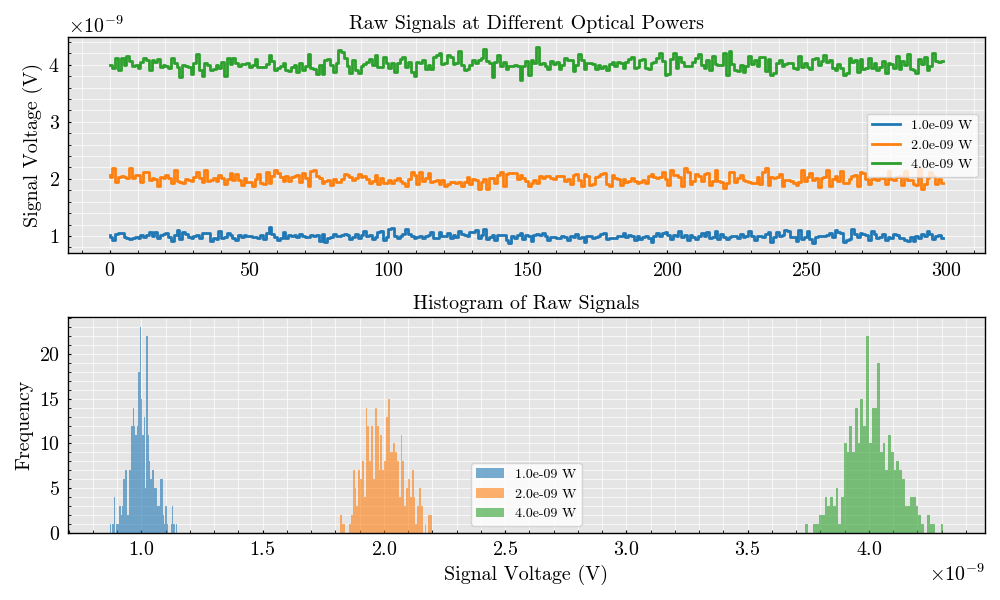
Shot noise

This example demonstrates the effect of different optical power levels on a flow cytometer detector. We initialize the detector, apply varying optical power levels, and visualize the resulting signals and their distributions.

import matplotlib.pyplot as plt
from FlowCyPy.detector import Detector
from FlowCyPy import units
import numpy
from FlowCyPy import SimulationSettings
from FlowCyPy.signal_generator import SignalGenerator

SimulationSettings.include_noises = True
SimulationSettings.include_shot_noise = True
SimulationSettings.include_dark_current_noise = False
SimulationSettings.include_source_noise = False

# Define optical power levels
optical_powers = [1 * units.nanowatt, 2 * units.nanowatt, 4 * units.nanowatt]  # Powers in watts
sequence_length = 300

Create a figure for signal visualization

fig, (ax_signal, ax_hist) = plt.subplots(2, 1, figsize=(10, 6), sharex=False)

# Loop over the optical power levels
for optical_power in optical_powers:
    detector_name = f"{optical_power.magnitude:.1e} W"

    signal_generator = SignalGenerator(n_elements=sequence_length, time_units=units.second, signal_units=units.watt)

    signal_generator.create_zero_signal(detector_name)

    signal_generator.add_constant(
        signal_name=detector_name,
        constant=optical_power.to('watt')
    )

    # Initialize the detector
    detector = Detector(
        name=detector_name,
        responsivity=1 * units.ampere / units.watt,
        numerical_aperture=0.2 * units.AU,
        phi_angle=0 * units.degree
    )

    detector.apply_shot_noise(
        signal_generator=signal_generator,
        wavelength=1550 * units.nanometer,
        bandwidth=10 * units.megahertz
    )

    noise_current = signal_generator.get_signal(detector_name) * units.ampere

    # Plot the raw signal on the first axis
    ax_signal.step(numpy.arange(sequence_length), noise_current, label=detector.name)

    # Plot the histogram of the raw signal
    ax_hist.hist(noise_current, bins=50, alpha=0.6, label=detector.name)

# Customize the axes
ax_signal.set_title("Raw Signals at Different Optical Powers")
ax_signal.set_ylabel("Signal Voltage (V)")
ax_signal.legend()

ax_hist.set_title("Histogram of Raw Signals")
ax_hist.set_xlabel("Signal Voltage (V)")
ax_hist.set_ylabel("Frequency")
ax_hist.legend()


# Show the plots
plt.tight_layout()
_ = plt.show()