
Note
Go to the end to download the full example code.
Flow Cytometry Workflow: Single Population Example#
This tutorial demonstrates a basic flow cytometry simulation using the FlowCyPy library.
The example covers the configuration of: - A fluidic channel with hydrodynamic focusing - A synthetic particle population (Exosome + HDL) - A laser source and dual-detector optical system - Scattering intensity calculation per detector
The resulting data are visualized using event-based plots.
Workflow Steps:#
Define laser source and flow cell geometry
Add synthetic particle populations
Model optical scattering with two detectors
Visualize population and scattering response
Step 0: Imports and Setup#
from TypedUnit import ureg

from FlowCyPy import OptoElectronics
from FlowCyPy.instances.detector import PMT
from FlowCyPy.instances.population import Exosome
from FlowCyPy.fluidics import FlowCell, Fluidics, ScattererCollection, population
from FlowCyPy.opto_electronics import TransimpedanceAmplifier, source
from FlowCyPy.signal_processing import Digitizer
Step 1: Define Optical Source#
laser = source.GaussianBeam(
    numerical_aperture=0.3 * ureg.AU,
    wavelength=750 * ureg.nanometer,
    optical_power=20 * ureg.milliwatt,
)
Step 2: Configure Flow Cell and Fluidics#
flow_cell = FlowCell(
    sample_volume_flow=0.02 * ureg.microliter / ureg.second,
    sheath_volume_flow=0.1 * ureg.microliter / ureg.second,
    width=20 * ureg.micrometer,
    height=10 * ureg.micrometer,
)

scatterer_collection = ScattererCollection(medium_refractive_index=1.33 * ureg.RIU)

# Add Exosome and HDL populations
scatterer_collection.add_population(
    Exosome(particle_count=5e10 * ureg.particle / ureg.milliliter),
)

fluidics = Fluidics(scatterer_collection=scatterer_collection, flow_cell=flow_cell)
Step 3: Generate Particle Event DataFrame#
event_frame = fluidics.generate_event_frame(run_time=3.5 * ureg.millisecond)
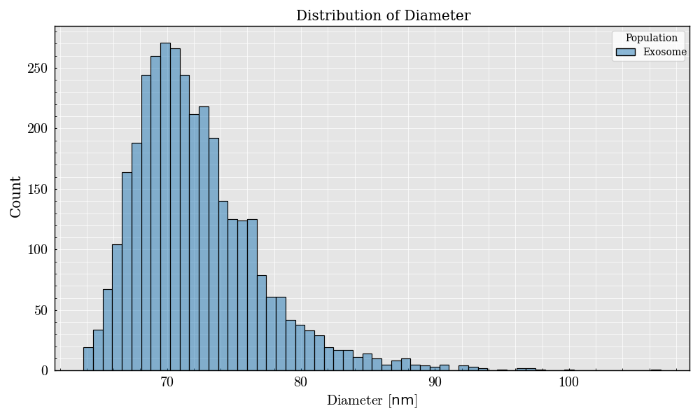
# Plot the diameter distribution of the particles
event_frame.plot(x="Diameter", bins="auto")
<Figure size 800x500 with 1 Axes>
Step 4: Define Detectors and Amplifier#
detector_forward = PMT(
    name="forward", phi_angle=0 * ureg.degree, numerical_aperture=0.3 * ureg.AU
)

detector_side = PMT(
    name="side", phi_angle=90 * ureg.degree, numerical_aperture=0.3 * ureg.AU
)

amplifier = TransimpedanceAmplifier(
    gain=100 * ureg.volt / ureg.ampere, bandwidth=10 * ureg.megahertz
)
Step 5: Configure Digitizer and Opto-Electronics#
digitizer = Digitizer(
    bit_depth="14bit", saturation_levels="auto", sampling_rate=60 * ureg.megahertz
)

opto_electronics = OptoElectronics(
    detectors=[detector_forward, detector_side], source=laser, amplifier=amplifier
)
Step 6: Model Scattering Signals#
opto_electronics.add_model_to_event_frame(
    event_frame=event_frame, compute_cross_section=True
)
/opt/hostedtoolcache/Python/3.11.14/x64/lib/python3.11/site-packages/FlowCyPy/source.py:268: UserWarning: Transverse distribution of particle flow exceed the waist of the source
  warnings.warn(
/opt/hostedtoolcache/Python/3.11.14/x64/lib/python3.11/site-packages/FlowCyPy/source.py:268: UserWarning: Transverse distribution of particle flow exceed the waist of the source
  warnings.warn(

<FlowCyPy.event_frame.EventFrame object at 0x7fa9b0c7c110>
Step 7: Visualize Scattering Intensity#
event_frame.plot(x="side", y="Csca") # Color-coded by scattering cross-section
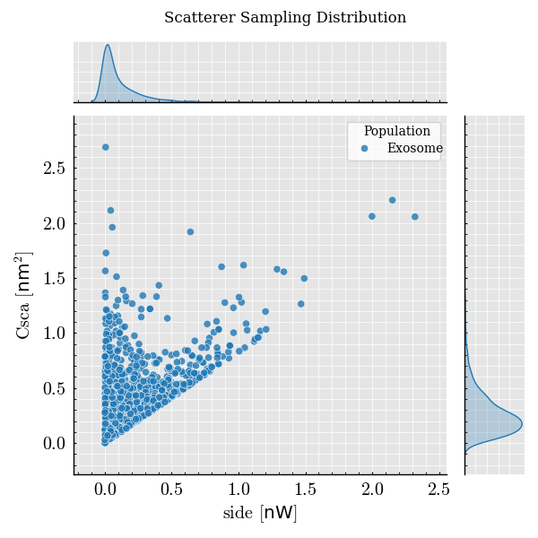
<Figure size 600x600 with 3 Axes>
Total running time of the script: (0 minutes 3.234 seconds)