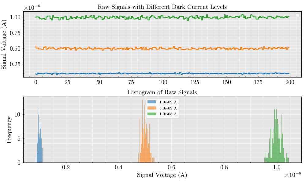
Dark Current

This example illustrates the impact of varying dark current levels on a flow cytometer detector signal. The detector is initialized, dark current noise is applied, and the resulting signals are visualized along with their distributions.

/home/runner/work/FlowCyPy/FlowCyPy/docs/examples/noise_sources/dark_current.py:52: UserWarning: No artists with labels found to put in legend.  Note that artists whose label start with an underscore are ignored when legend() is called with no argument.
  ax_signal.legend()

import matplotlib.pyplot as plt
from FlowCyPy.detector import Detector
from FlowCyPy import units
from FlowCyPy import TransimpedanceAmplifier
import numpy
from FlowCyPy import NoiseSetting

NoiseSetting.include_noises = True
NoiseSetting.include_shot_noise = False
NoiseSetting.include_dark_current_noise = True
NoiseSetting.include_source_noise = False

# Define dark current levels
dark_currents = [1e-9 * units.ampere, 5e-9 * units.ampere, 1e-8 * units.ampere]  # Dark current levels in amperes

# Create a figure for signal visualization
fig, (ax_signal, ax_hist) = plt.subplots(2, 1, figsize=(10, 6), sharex=False)

# Loop over the dark current levels
for dark_current in dark_currents:
    # Initialize the detector
    detector = Detector(
        name=f"{dark_current.magnitude:.1e} A",
        responsivity=1 * units.ampere / units.watt,  # Responsitivity (current per power)
        numerical_aperture=0.2 * units.AU,      # Numerical aperture
        phi_angle=0 * units.degree,             # Detector orientation angle
        dark_current=dark_current         # Dark current level
    )

    # Add dark current noise to the raw signal
    noise_current = detector.get_dark_current_noise(sequence_length=200, bandwidth=10 * units.megahertz).to(units.ampere)

    # Plot the raw signal on the first axis
    ax_signal.step(x=numpy.arange(200), y=noise_current)

    # Plot the histogram of the raw signal
    ax_hist.hist(noise_current, bins=50, alpha=0.6, label=detector.name)

# Customize the axes
ax_signal.set_title("Raw Signals with Different Dark Current Levels")
ax_signal.set_ylabel("Signal Voltage (A)")
ax_signal.legend()

ax_hist.set_title("Histogram of Raw Signals")
ax_hist.set_xlabel("Signal Voltage (A)")
ax_hist.set_ylabel("Frequency")
ax_hist.legend()

# Show the plots
plt.tight_layout()
plt.show()