Signal Processing in Flow Cytometry

This example demonstrates how to apply signal processing techniques to flow cytometry data using FlowCyPy. The simulation is set up with a Gaussian beam, a flow cell, and two detectors. A single population of scatterers (with delta distributions) is used, and the focus here is on processing the forward scatter detector signals. Three acquisitions are performed:

• Raw Signal: No processing applied.

• Baseline Restored: Using a baseline restorator.

• Bessel LowPass: Using a Bessel low-pass filter.

The resulting signals are plotted for comparison.

import numpy as np
import matplotlib.pyplot as plt

# Import necessary components from FlowCyPy
from FlowCyPy import (
    FlowCytometer, ScattererCollection, Detector, GaussianBeam,
    population, distribution, circuits, units, NoiseSetting, TransimpedanceAmplifier
)
from FlowCyPy.flow_cell import FlowCell
from FlowCyPy.signal_digitizer import SignalDigitizer

# Enable noise settings if desired
NoiseSetting.include_noises = True

# Set random seed for reproducibility
np.random.seed(3)

# Define the optical source: a Gaussian beam.
source = GaussianBeam(
    numerical_aperture=0.3 * units.AU,            # Numerical aperture of the laser
    wavelength=488 * units.nanometer,             # Laser wavelength: 488 nm
    optical_power=100 * units.milliwatt           # Laser optical power: 100 mW
)

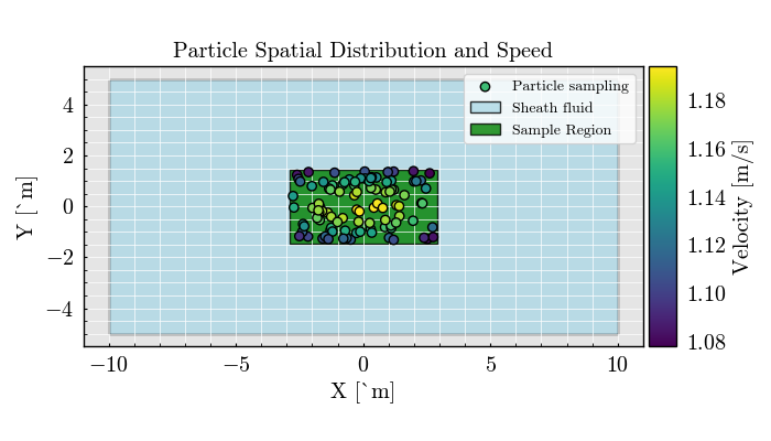
Define and plot the flow cell.

flow_cell = FlowCell(
    sample_volume_flow=0.02 * units.microliter / units.second,
    sheath_volume_flow=0.1 * units.microliter / units.second,
    width=20 * units.micrometer,
    height=10 * units.micrometer,
)

flow_cell.plot(n_samples=100)


# Create a scatterer collection with a single population.
# For signal processing, we use delta distributions (i.e., no variability).
population = population.Sphere(
    name='Population',
    particle_count=10 * units.particle,
    diameter=distribution.Delta(position=150 * units.nanometer),
    refractive_index=distribution.Delta(position=1.39 * units.RIU)
)
scatterer_collection = ScattererCollection(
    medium_refractive_index=1.33 * units.RIU,
    populations=[population]
)

# Define the signal digitizer.
digitizer = SignalDigitizer(
    bit_depth='14bit',
    saturation_levels='auto',
    sampling_rate=60 * units.megahertz  # Sampling rate: 60 MHz
)

# Define two detectors.
detector_0 = Detector(
    name='side',
    phi_angle=90 * units.degree,
    numerical_aperture=0.2 * units.AU,
    responsivity=1 * units.ampere / units.watt,
    dark_current=10 * units.microampere,
)

detector_1 = Detector(
    name='forward',
    phi_angle=0 * units.degree,
    numerical_aperture=0.2 * units.AU,
    responsivity=1 * units.ampere / units.watt,
    dark_current=1 * units.microampere,
)

transimpedance_amplifier = TransimpedanceAmplifier(
    gain=100 * units.volt / units.ampere,
    bandwidth = 10 * units.megahertz
)

# Setup the flow cytometer.
cytometer = FlowCytometer(
    source=source,
    transimpedance_amplifier=transimpedance_amplifier,
    digitizer=digitizer,
    scatterer_collection=scatterer_collection,
    flow_cell=flow_cell,
    background_power=2 * units.microwatt,
    detectors=[detector_0, detector_1]
)

# ---------------------------------------------------------------------------
# Signal Processing: Acquisition with Different Processing Steps
# ---------------------------------------------------------------------------

fig, ax = plt.subplots(1, 1, figsize=(12, 6))

# Acquisition 1: Raw Signal (no processing)
processing_steps_none = []
cytometer.prepare_acquisition(run_time=0.1 * units.millisecond)
acquisition_none = cytometer.get_acquisition(processing_steps=processing_steps_none)
ax.plot(
    acquisition_none['Time'].pint.to('microsecond'),
    acquisition_none['forward'].pint.to('millivolt'),
    linestyle='-',
    label='Raw Signal'
)

# Acquisition 2: Baseline Restoration
processing_steps_baseline = [circuits.BaselineRestorator(window_size=1000 * units.microsecond)]
acquisition_baseline = cytometer.get_acquisition(processing_steps=processing_steps_baseline)
ax.plot(
    acquisition_baseline['Time'].pint.to('microsecond'),
    acquisition_baseline['forward'].pint.to('millivolt'),
    linestyle='--',
    label='Baseline Restored'
)

# Acquisition 3: Bessel LowPass Filter
processing_steps_bessel = [circuits.BesselLowPass(cutoff=3 * units.megahertz, order=4, gain=2)]
acquisition_bessel = cytometer.get_acquisition(processing_steps=processing_steps_bessel)
ax.plot(
    acquisition_bessel['Time'].pint.to('microsecond'),
    acquisition_bessel['forward'].pint.to('millivolt'),
    linestyle='-.',
    label='Bessel LowPass'
)

# Configure the plot.
ax.set_title("Flow Cytometry Signal Processing")
ax.set_xlabel("Time [microsecond]")
ax.set_ylabel("Signal Amplitude [millivolt]")
ax.legend()
plt.tight_layout()
plt.show()

• 
• 

/opt/hostedtoolcache/Python/3.11.12/x64/lib/python3.11/site-packages/FlowCyPy/source.py:269: UserWarning: Transverse distribution of particle flow exceed the waist of the source
  warnings.warn('Transverse distribution of particle flow exceed the waist of the source')
/opt/hostedtoolcache/Python/3.11.12/x64/lib/python3.11/site-packages/FlowCyPy/source.py:269: UserWarning: Transverse distribution of particle flow exceed the waist of the source
  warnings.warn('Transverse distribution of particle flow exceed the waist of the source')