Limit of Detection

This example simulates the detection of small nanoparticles (90–150 nm diameter) in a flow cytometry setup using a dual-detector configuration (side and forward scatter). The simulation includes noise models, realistic fluidics, analog signal conditioning, digitization, triggering, and peak detection.

The main goal is to evaluate whether such particles produce detectable and distinguishable scatter signals in the presence of system noise and fluidic variability.

import numpy as np
from TypedUnit import ureg

from FlowCyPy import FlowCytometer, SimulationSettings
from FlowCyPy.fluidics import (
    FlowCell,
    Fluidics,
    ScattererCollection,
    distribution,
    population,
)
from FlowCyPy.opto_electronics import (
    Detector,
    OptoElectronics,
    TransimpedanceAmplifier,
    source,
)
from FlowCyPy.signal_processing import (
    Digitizer,
    SignalProcessing,
    circuits,
    peak_locator,
    triggering_system,
)

Simulation Configuration

SimulationSettings.include_noises = True
SimulationSettings.include_shot_noise = True
SimulationSettings.include_source_noise = True
SimulationSettings.include_dark_current_noise = True
SimulationSettings.assume_perfect_hydrodynamic_focusing = True
SimulationSettings.evenly_spaced_events = True
SimulationSettings.sorted_population = True

np.random.seed(3)

Optical Source

source = source.GaussianBeam(
    numerical_aperture=0.1 * ureg.AU,
    wavelength=488 * ureg.nanometer,
    optical_power=200 * ureg.milliwatt,
)

Flow Cell Configuration

flow_cell = FlowCell(
    sample_volume_flow=0.02 * ureg.microliter / ureg.second,
    sheath_volume_flow=0.1 * ureg.microliter / ureg.second,
    width=20 * ureg.micrometer,
    height=10 * ureg.micrometer,
)

Define Scatterer Populations (90–150 nm spheres)

scatterer_collection = ScattererCollection(medium_refractive_index=1.33 * ureg.RIU)

for size in [150, 130, 110, 90]:
    pop = population.Sphere(
        name=f"{size} nm",
        particle_count=20 * ureg.particle,
        diameter=distribution.Delta(position=size * ureg.nanometer),
        refractive_index=distribution.Delta(position=1.39 * ureg.RIU),
    )
    scatterer_collection.add_population(pop)

Fluidics Subsystem

fluidics = Fluidics(scatterer_collection=scatterer_collection, flow_cell=flow_cell)

Signal Digitizer

digitizer = Digitizer(
    bit_depth="14bit", saturation_levels="auto", sampling_rate=60 * ureg.megahertz
)

Detectors

detector_side = Detector(
    name="side",
    phi_angle=90 * ureg.degree,
    numerical_aperture=0.2 * ureg.AU,
    responsivity=1 * ureg.ampere / ureg.watt,
    dark_current=0.001 * ureg.milliampere,
)

detector_forward = Detector(
    name="forward",
    phi_angle=0 * ureg.degree,
    numerical_aperture=0.2 * ureg.AU,
    responsivity=1 * ureg.ampere / ureg.watt,
    dark_current=0.001 * ureg.milliampere,
)

Amplifier and Opto-Electronics

amplifier = TransimpedanceAmplifier(
    gain=10000 * ureg.volt / ureg.ampere, bandwidth=10 * ureg.megahertz
)

opto_electronics = OptoElectronics(
    detectors=[detector_side, detector_forward], source=source, amplifier=amplifier
)

Analog Processing Pipeline

analog_processing = [
    circuits.BaselineRestorator(window_size=10 * ureg.microsecond),
    circuits.BesselLowPass(cutoff=1 * ureg.megahertz, order=4, gain=2),
]

Triggering and Peak Detection

triggering_system = triggering_system.DynamicWindow(
    trigger_detector_name="forward",
    threshold=0.4 * ureg.millivolt,
    max_triggers=-1,
    pre_buffer=64,
    post_buffer=64,
)

signal_processing = SignalProcessing(
    digitizer=digitizer,
    analog_processing=analog_processing,
    triggering_system=triggering_system,
    peak_algorithm=peak_locator.GlobalPeakLocator(),
)

cytometer = FlowCytometer(
    opto_electronics=opto_electronics,
    fluidics=fluidics,
    signal_processing=signal_processing,
    background_power=0.0001 * ureg.milliwatt,
)

results = cytometer.run(run_time=1.0 * ureg.millisecond)

Population  ScattererID
150 nm      0               0.0
            1              -0.0
            2              -0.0
            3              -0.0
            4              -0.0
                           ...
90 nm       14              0.0
            15              0.0
            16              0.0
            17              0.0
            18             -0.0
Name: y, Length: 86, dtype: pint[meter][Float64] 1553.3522445768986 nanometer
Population  ScattererID
150 nm      0               0.0
            1              -0.0
            2              -0.0
            3              -0.0
            4              -0.0
                           ...
90 nm       14              0.0
            15              0.0
            16              0.0
            17              0.0
            18             -0.0
Name: y, Length: 86, dtype: pint[meter][Float64] 1553.3522445768986 nanometer

Plot Raw Analog Signal

results.analog.normalize_units(time_units="max", signal_units="max")
results.analog.plot()

• 
• 

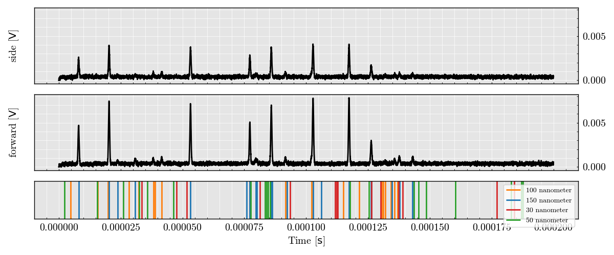
<Figure size 1200x500 with 1 Axes>

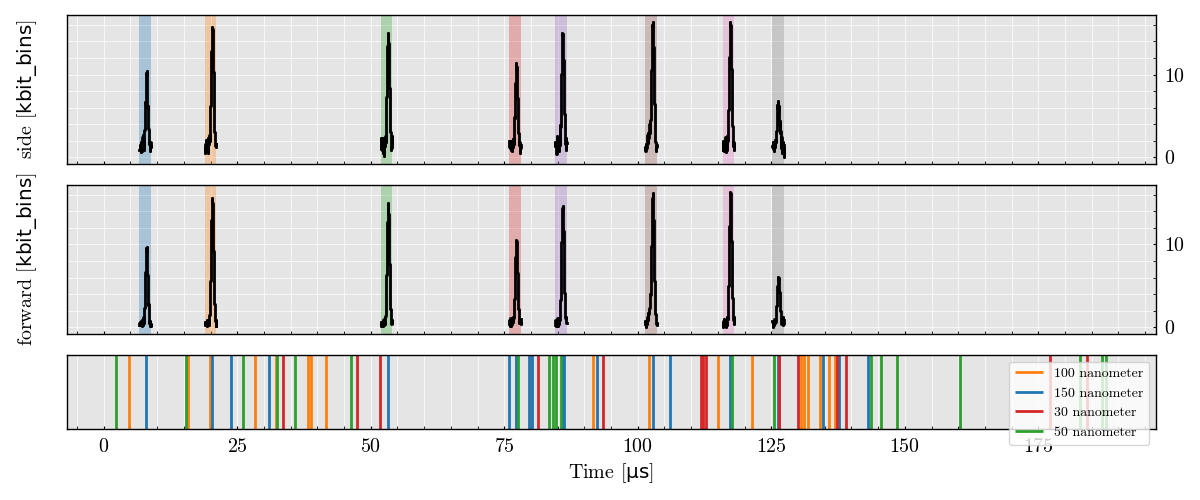
Plot Triggered Analog Signal Segments

results.triggered_analog.plot()

• 
• 

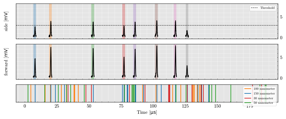
<Figure size 1200x500 with 1 Axes>

Plot Peak Features (Side vs Forward Height)

results.peaks.plot(x=("side", "Height"), y=("forward", "Height"))

<seaborn.axisgrid.JointGrid object at 0x7f8a3e408a90>