Generating Signal

This script simulates signals from a flow cytometer using Rayleigh scattering to model the interaction of particles with a laser beam. It demonstrates how to generate Forward Scatter (FSC) and Side Scatter (SSC) signals using FlowCyPy and visualize the results.

Steps: 1. Define the flow parameters and particle size distribution. 2. Set up the laser source and detectors. 3. Simulate the flow cytometer signals. 4. Visualize and analyze the signals from FSC and SSC detectors.

# Step 1: Import the necessary libraries
from FlowCyPy import FlowCytometer, ScattererCollection, Detector, GaussianBeam, TransimpedanceAmplifier
from FlowCyPy import distribution, population
from FlowCyPy.flow_cell import FlowCell
from FlowCyPy.signal_digitizer import SignalDigitizer
from FlowCyPy import units

# Step 2: Set up the light source
# -------------------------------
# A laser with a wavelength of 1550 nm, optical power of 2 mW, and a numerical aperture of 0.4 is used.
source = GaussianBeam(
    numerical_aperture=0.4 * units.AU,     # Numerical aperture: 0.4
    wavelength=1550 * units.nanometer,     # Wavelength: 1550 nm
    optical_power=200 * units.milliwatt    # Optical power: 2 mW
)

# Step 3: Define the flow parameters
# ----------------------------------
# Flow speed is set to 80 micrometers per second, with a flow area of 1 square micrometer and a total simulation time of 1 second.
flow_cell = FlowCell(
    sample_volume_flow=0.02 * units.microliter / units.second,        # Flow speed: 10 microliter per second
    sheath_volume_flow=0.1 * units.microliter / units.second,        # Flow speed: 10 microliter per second
    width=20 * units.micrometer,        # Flow area: 10 x 10 micrometers
    height=10 * units.micrometer,        # Flow area: 10 x 10 micrometers
)

# Step 4: Define the particle size distribution
# ---------------------------------------------
# We define a normal distribution for particle sizes with a mean of 200 nm, standard deviation of 10 nm,
# and a refractive index of 1.39 with a small variation of 0.01.
scatterer_collection = ScattererCollection(medium_refractive_index=1.33 * units.RIU)

population_0 = population.Sphere(
    name='EV',
    particle_count=1e+9 * units.particle / units.milliliter,
    diameter=distribution.RosinRammler(characteristic_property=200 * units.nanometer, spread=4.5),
    refractive_index=distribution.Normal(mean=1.42 * units.RIU, std_dev=0.05 * units.RIU)
)

population_1 = population.Sphere(
    name='LP',
    particle_count=1e+11 * units.particle / units.milliliter,
    diameter=distribution.RosinRammler(characteristic_property=100 * units.nanometer, spread=4.5),
    refractive_index=distribution.Normal(mean=1.39 * units.RIU, std_dev=0.05 * units.RIU)
)

scatterer_collection.add_population(population_1, population_0)

# scatterer_collection.dilute(100)

# Step 5: Set up the detectors
# ----------------------------
# Two detectors are used: Forward Scatter (FSC) and Side Scatter (SSC). Each detector is configured
# with its own numerical aperture, responsivity, noise level, and acquisition frequency.
digitizer = SignalDigitizer(
    bit_depth=1024,
    saturation_levels='auto',
    sampling_rate=10 * units.megahertz,           # Sampling frequency: 10 MHz
)

detector_fsc = Detector(
    name='FSC',                         # Forward Scatter detector
    numerical_aperture=1.2 * units.AU,        # Numerical aperture: 0.2
    phi_angle=0 * units.degree,               # Angle: 180 degrees for forward scatter
)

detector_ssc = Detector(
    name='SSC',                         # Side Scatter detector
    numerical_aperture=1.2 * units.AU,        # Numerical aperture: 0.2
    phi_angle=90 * units.degree,              # Angle: 90 degrees for side scatter
)

transimpedance_amplifier = TransimpedanceAmplifier(
    gain=100 * units.volt / units.ampere,
    bandwidth = 10 * units.megahertz
)


# Step 6: Create a FlowCytometer instance
# ---------------------------------------
# The flow cytometer is configured with the source, scatterer distribution, and detectors.
# The 'mie' coupling mechanism models how the particles interact with the laser beam.
cytometer = FlowCytometer(
    source=source,
    transimpedance_amplifier=transimpedance_amplifier,
    digitizer=digitizer,
    scatterer_collection=scatterer_collection,
    flow_cell=flow_cell,  # Particle size distribution
    detectors=[detector_fsc, detector_ssc],  # Detectors: FSC and SSC
)

# Step 7: Simulate flow cytometer signals
# ---------------------------------------
# Simulate the signals for both detectors (FSC and SSC) as particles pass through the laser beam.
# Run the flow cytometry simulation
acquisition = cytometer.prepare_acquisition(run_time=0.2 * units.millisecond)
acquisition = cytometer.get_acquisition()



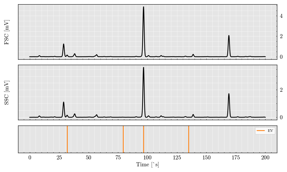
# Visualize the scatter signals from both detectors
acquisition.plot(filter_population=['EV'])



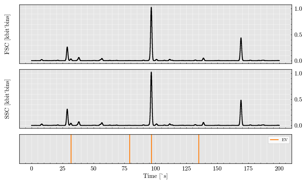
digital_signal = acquisition.digitalize(digitizer=digitizer)
digital_signal.plot(filter_population=['EV'])

• 
• 

/opt/hostedtoolcache/Python/3.11.12/x64/lib/python3.11/site-packages/FlowCyPy/source.py:269: UserWarning: Transverse distribution of particle flow exceed the waist of the source
  warnings.warn('Transverse distribution of particle flow exceed the waist of the source')
/opt/hostedtoolcache/Python/3.11.12/x64/lib/python3.11/site-packages/FlowCyPy/source.py:269: UserWarning: Transverse distribution of particle flow exceed the waist of the source
  warnings.warn('Transverse distribution of particle flow exceed the waist of the source')

The above plot shows the raw simulated signals for Forward Scatter (FSC) and Side Scatter (SSC) channels. These signals provide insights into particle size and complexity and can be further analyzed for feature extraction, such as peak height and width.