WorkFlow

This script simulates flow cytometer signals using the FlowCytometer class and analyzes the results using the PulseAnalyzer class from the FlowCyPy library. The signals generated (forward scatter and side scatter) provide insights into the physical properties of particles passing through the laser beam.

Workflow:

1. Define a particle size distribution using ScattererCollection.

2. Simulate flow cytometer signals using FlowCytometer.

3. Analyze the forward scatter signal with PulseAnalyzer to extract features like peak height, width, and area.

4. Visualize the generated signals and display the extracted pulse features.

Step 1: Import necessary modules from FlowCyPy

from FlowCyPy import FlowCytometer, ScattererCollection, Detector, GaussianBeam, TransimpedanceAmplifier
from FlowCyPy import distribution
from FlowCyPy.population import Sphere
from FlowCyPy.signal_digitizer import SignalDigitizer
from FlowCyPy.flow_cell import FlowCell
from FlowCyPy import units
from FlowCyPy.triggering_system import TriggeringSystem

import numpy
numpy.random.seed(3)

Step 2: Define the laser source

Set up a laser source with a wavelength of 1550 nm, optical power of 200 mW, and a numerical aperture of 0.3.

source = GaussianBeam(
    numerical_aperture=0.3 * units.AU,  # Numerical aperture: 0.3
    wavelength=800 * units.nanometer,   # Laser wavelength: 800 nm
    optical_power=20 * units.milliwatt  # Optical power: 20 milliwatts
)

Step 3: Define flow parameters

Set the flow speed to 80 micrometers per second and a flow area of 1 square micrometer, with a total simulation time of 1 second.

flow_cell = FlowCell(
    sample_volume_flow=0.02 * units.microliter / units.second,        # Flow speed: 10 microliter per second
    sheath_volume_flow=0.1 * units.microliter / units.second,        # Flow speed: 10 microliter per second
    width=20 * units.micrometer,        # Flow area: 10 x 10 micrometers
    height=10 * units.micrometer,        # Flow area: 10 x 10 micrometers
)

Step 4: Define the particle size distribution

Use a normal size distribution with a mean size of 200 nanometers and a standard deviation of 10 nanometers. This represents the population of scatterers (particles) that will interact with the laser source.

ev_diameter = distribution.Normal(
    mean=200 * units.nanometer,       # Mean particle size: 200 nanometers
    std_dev=10 * units.nanometer      # Standard deviation: 10 nanometers
)

ev_ri = distribution.Normal(
    mean=1.39 * units.RIU,    # Mean refractive index: 1.39
    std_dev=0.01 * units.RIU  # Standard deviation: 0.01
)

ev = Sphere(
    particle_count=20 * units.particle,
    diameter=ev_diameter,               # Particle size distribution
    refractive_index=ev_ri,     # Refractive index distribution
    name='EV'                   # Name of the particle population: Extracellular Vesicles (EV)
)

scatterer_collection = ScattererCollection()

scatterer_collection.add_population(ev)

scatterer_collection.dilute(2)

# Step 5: Define the detector
# ---------------------------
# The detector captures the scattered light. It is positioned at 90 degrees relative to the incident light beam
# and configured with a numerical aperture of 0.4 and responsivity of 1.
digitizer = SignalDigitizer(
    bit_depth=1024,
    saturation_levels='auto',
    sampling_rate=10 * units.megahertz,        # Sampling frequency: 1 MHz
)

detector_0 = Detector(
    phi_angle=90 * units.degree,              # Detector angle: 90 degrees (Side Scatter)
    numerical_aperture=0.4 * units.AU,        # Numerical aperture of the detector
    name='side',              # Detector name
    responsivity=1 * units.ampere / units.watt,   # Responsitivity of the detector (light to signal conversion efficiency)
)

detector_1 = Detector(
    phi_angle=0 * units.degree,               # Detector angle: 90 degrees (Sid e Scatter)
    numerical_aperture=0.4 * units.AU,        # Numerical aperture of the detector
    name='forward',             # Detector name
    responsivity=1 * units.ampere / units.watt,   # Responsitivity of the detector (light to signal conversion efficiency)
)

transimpedance_amplifier = TransimpedanceAmplifier(
    gain=100 * units.volt / units.ampere,
    bandwidth = 10 * units.megahertz
)

# Step 6: Simulate Flow Cytometer Signals
# ---------------------------------------
# Create a FlowCytometer instance to simulate the signals generated as particles pass through the laser beam.
cytometer = FlowCytometer(
    source=source,
    transimpedance_amplifier=transimpedance_amplifier,
    digitizer=digitizer,
    background_power=0.01 * units.milliwatt,
    scatterer_collection=scatterer_collection,
    flow_cell=flow_cell,                # Particle size distribution
    detectors=[detector_0, detector_1]  # List of detectors used in the simulation
)

# Run the flow cytometry simulation
acquisition = cytometer.prepare_acquisition(run_time=0.3 * units.millisecond)
acquisition = cytometer.get_acquisition()

/opt/hostedtoolcache/Python/3.11.12/x64/lib/python3.11/site-packages/FlowCyPy/source.py:269: UserWarning: Transverse distribution of particle flow exceed the waist of the source
  warnings.warn('Transverse distribution of particle flow exceed the waist of the source')
/opt/hostedtoolcache/Python/3.11.12/x64/lib/python3.11/site-packages/FlowCyPy/source.py:269: UserWarning: Transverse distribution of particle flow exceed the waist of the source
  warnings.warn('Transverse distribution of particle flow exceed the waist of the source')

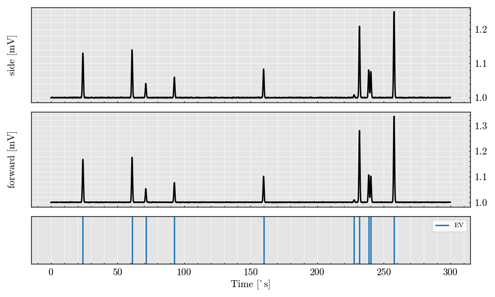
Visualize the scatter analog signals from both detectors

acquisition.plot()

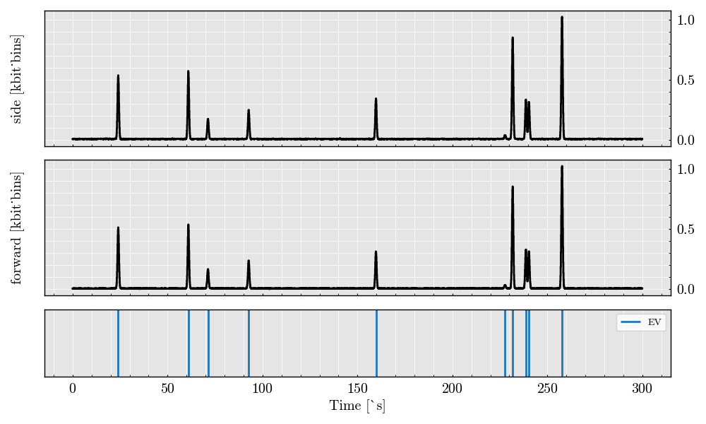
Visualize the scatter digital signals from both detectors

digital_signal = acquisition.digitalize(digitizer=digitizer)
digital_signal.plot()

trigger = TriggeringSystem(
    threshold='3 sigma',
    max_triggers=-1,
    pre_buffer=20,
    post_buffer=20,
    digitizer=digitizer
)

analog_triggered = trigger.run(
    signal_dataframe=acquisition,
    trigger_detector_name='forward',
)

# # %%
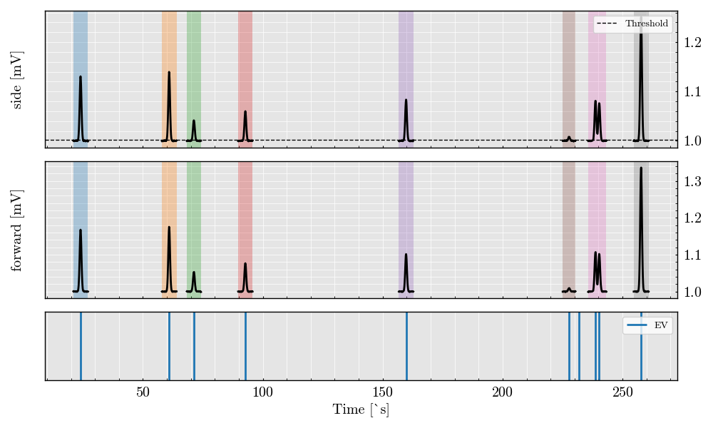
# # Visualize the scatter triggered analog signals from both detectors
analog_triggered.plot()

# # %%
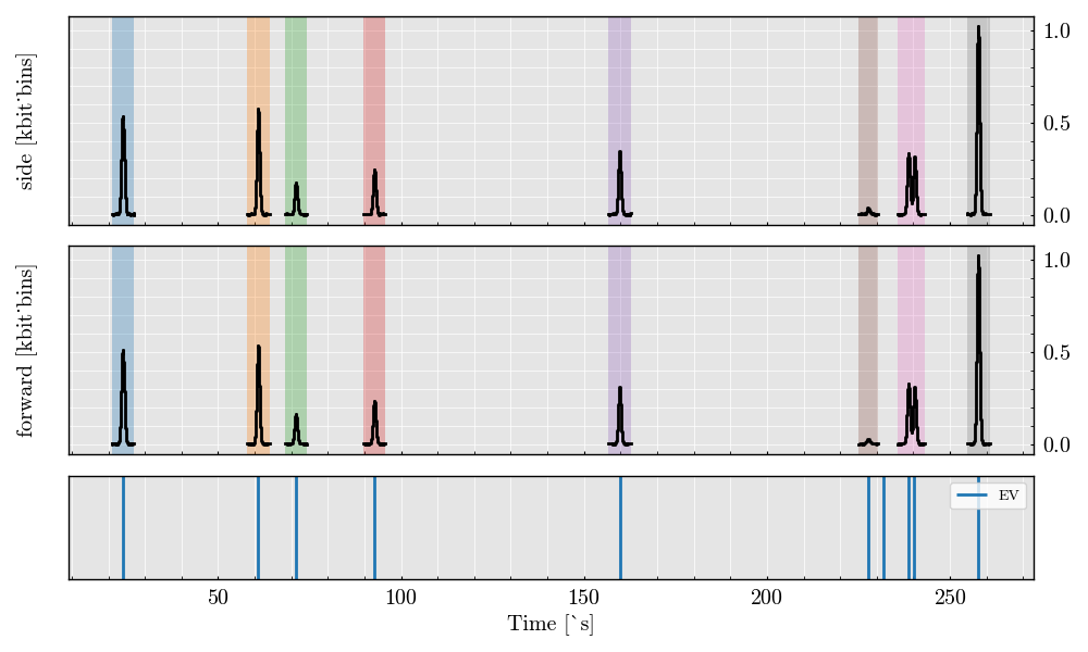
# # Visualize the scatter triggered digital signals from both detectors
digital_triggered = analog_triggered.digitalize(digitizer=digitizer)
digital_triggered.plot()

• 
• 
•