Workflow

This tutorial demonstrates how to simulate a flow cytometry experiment using the FlowCyPy library. The simulation involves configuring a flow setup, defining a single population of particles, and analyzing scattering signals from two detectors to produce a 2D density plot of scattering intensities.

Overview:

1. Configure the flow cell and particle population.

2. Define the laser source and detector parameters.

3. Simulate the flow cytometry experiment.

4. Analyze the generated signals and visualize results.

Step 0: Import Necessary Libraries

Here, we import the necessary libraries and units for the simulation. The units module helps us define physical quantities like meters, seconds, and watts in a concise and consistent manner.

from FlowCyPy import units
from FlowCyPy import GaussianBeam
from FlowCyPy.flow_cell import FlowCell
from FlowCyPy import ScattererCollection
from FlowCyPy.population import Exosome, HDL
from FlowCyPy.detector import PMT
from FlowCyPy.signal_digitizer import SignalDigitizer
from FlowCyPy import FlowCytometer, TransimpedanceAmplifier

source = GaussianBeam(
    numerical_aperture=0.3 * units.AU,           # Numerical aperture
    wavelength=200 * units.nanometer,           # Wavelength
    optical_power=20 * units.milliwatt          # Optical power
)

flow_cell = FlowCell(
    sample_volume_flow=0.02 * units.microliter / units.second,
    sheath_volume_flow=0.1 * units.microliter / units.second,
    width=20 * units.micrometer,
    height=10 * units.micrometer,
)

scatterer_collection = ScattererCollection(medium_refractive_index=1.33 * units.RIU)

# Add an Exosome and HDL population
scatterer_collection.add_population(
    Exosome(particle_count=5e9 * units.particle / units.milliliter),
    HDL(particle_count=5e9 * units.particle / units.milliliter)
)

scatterer_collection.dilute(factor=1)

# Initialize the scatterer with the flow cell
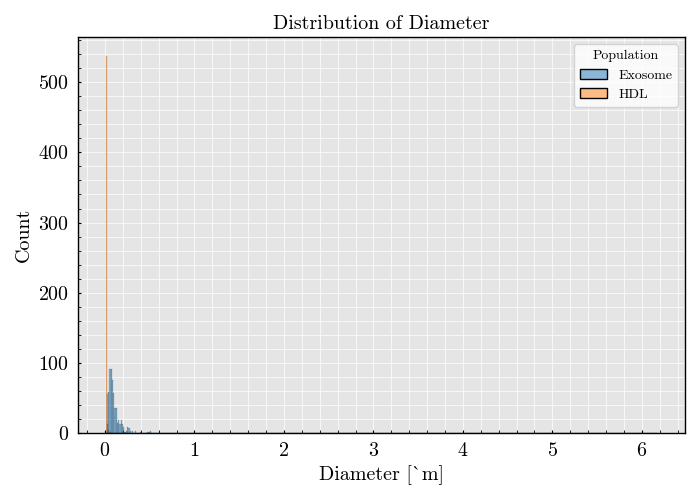
df = scatterer_collection.get_population_dataframe(total_sampling=600, use_ratio=False)  # Visualize the particle population

df.plot(x='Diameter', bins='auto')

digitizer = SignalDigitizer(
    bit_depth='14bit',
    saturation_levels='auto',
    sampling_rate=60 * units.megahertz,
)

detector_0 = PMT(name='forward', phi_angle=0 * units.degree, numerical_aperture=0.3 * units.AU)

detector_1 = PMT(name='side', phi_angle=90 * units.degree, numerical_aperture=0.3 * units.AU)

transimpedance_amplifier = TransimpedanceAmplifier(
    gain=100 * units.volt / units.ampere,
    bandwidth = 10 * units.megahertz
)


cytometer = FlowCytometer(
    source=source,
    transimpedance_amplifier=transimpedance_amplifier,
    scatterer_collection=scatterer_collection,
    digitizer=digitizer,
    detectors=[detector_0, detector_1],
    flow_cell=flow_cell,
    background_power=0.001 * units.milliwatt
)

# Run the flow cytometry simulation
cytometer.prepare_acquisition(run_time=0.1 * units.millisecond)

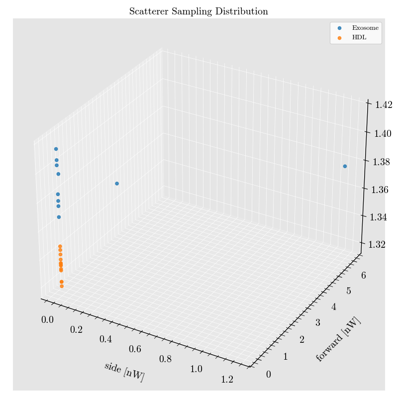
cytometer.scatterer_dataframe.plot(
    x='side',
    y='forward',
    z='RefractiveIndex'
)

• 
• 

/opt/hostedtoolcache/Python/3.11.12/x64/lib/python3.11/site-packages/FlowCyPy/source.py:269: UserWarning: Transverse distribution of particle flow exceed the waist of the source
  warnings.warn('Transverse distribution of particle flow exceed the waist of the source')
/opt/hostedtoolcache/Python/3.11.12/x64/lib/python3.11/site-packages/FlowCyPy/source.py:269: UserWarning: Transverse distribution of particle flow exceed the waist of the source
  warnings.warn('Transverse distribution of particle flow exceed the waist of the source')

<Figure size 800x800 with 1 Axes>