Monodisperse Percus–Yevick fluid at several densities

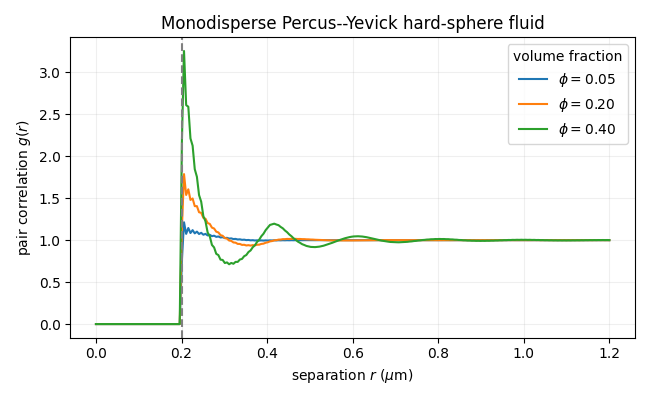
This example shows how the radial distribution function of an equilibrium hard-sphere fluid changes with volume fraction. At higher density, the first neighbour shell becomes more pronounced. Each curve is an independent Percus–Yevick calculation; it is not an RSA packing trajectory.

import matplotlib.pyplot as plt
import numpy as np

from PackLab import analytical, ureg

Solve a one-radius fluid for several volume fractions

radius = 100 * ureg.nanometer
distances = np.linspace(0.0, 1.2, 240) * ureg.micrometer
volume_fractions = (0.05, 0.20, 0.40)

figure, axis = plt.subplots(figsize=(6.5, 4))
for volume_fraction in volume_fractions:
    domain = analytical.PercusYevickDomain(
        size=50 * ureg.micrometer,
        radii=np.array([radius.magnitude]) * radius.units,
        volume_fraction=volume_fraction,
        number_fractions=np.array([1.0]),
    )
    result = analytical.PercusYevickSolver(
        densities=domain.particle_densities_per_radius,
        radii=domain.radii,
        wavenumber="auto",
    ).compute(distances)
    _ = axis.plot(
        distances.to("micrometer").magnitude,
        result.g[0, 0],
        label=rf"$\phi={volume_fraction:.2f}$",
    )

_ = axis.axvline(2 * radius.to("micrometer").magnitude, color="0.5", linestyle="--")
_ = axis.set(
    xlabel=r"separation $r$ ($\mu$m)",
    ylabel=r"pair correlation $g(r)$",
    title="Monodisperse Percus--Yevick hard-sphere fluid",
)
_ = axis.legend(title="volume fraction")
axis.grid(alpha=0.2)
figure.tight_layout()