Percus Yevick mixture solver workflow

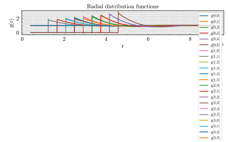
This example demonstrates the complete workflow for computing the radial distribution function \(g_{ij}(r)\) of a polydisperse hard sphere mixture using a Percus Yevick style solver.

The example covers the following steps:

1. Define a polydisperse domain (radii, volume fraction, number fractions)

2. Build the Fourier wavenumber grid

3. Construct the Percus Yevick solver

4. Compute reciprocal-space correlations and \(g_{ij}(r)\)

5. Plot all \(g_{ij}(r)\) curves on a single figure

The main output is a figure showing all pair correlations \(g_{ij}(r)\) for each species pair \((i, j)\).

import matplotlib.pyplot as plt
import numpy as np

from PackLab import ureg
from PackLab import analytical, samplers

distribution = samplers.NormalRadiusSampler(
    mean=1.5 * ureg.micrometer,
    standard_deviation=0.2 * ureg.micrometer,
    bins=6,
)

particle_radii, number_fractions = distribution.to_bins()

domain = analytical.PercusYevickDomain(
    size=100 * ureg.micrometer,
    radii=particle_radii,
    volume_fraction=0.3,
    number_fractions=number_fractions,
)

domain.print_bins()

distances = np.linspace(domain.radii.min() * 2, domain.radii.max() * 4, 1500)
solver = analytical.PercusYevickSolver(
    densities=domain.particle_densities_per_radius,
    radii=domain.radii,
    wavenumber="auto",
)

result = solver.compute(distances=distances)


figure, ax = plt.subplots(1, 1)

r = result.distances.magnitude
n = result.g.shape[0]


for i in range(n):
    for j in range(n):
        _ = ax.plot(
            result.distances.magnitude,
            result.g[i, j, :],
            label=f"g[{i},{j}]"
        )

ax.set_xlabel("r")
ax.set_ylabel("g(r)")
ax.set_title("Radial distribution functions")

_ = ax.legend()

plt.show()