PackLab monodisperse Percus–Yevick versus Tsang et al.

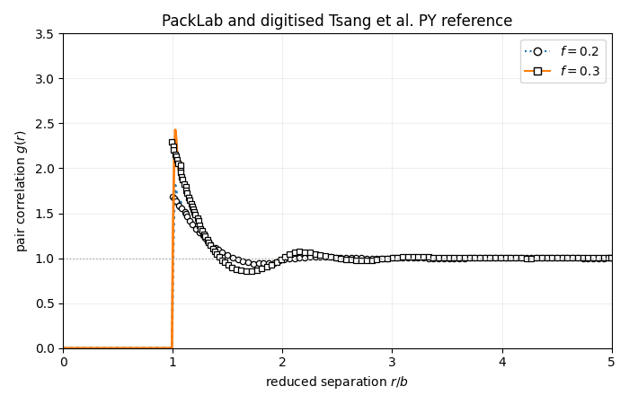
This example compares PackLab’s monodisperse Percus–Yevick (PY) solution with digitised PY curves from Figure 8.1.3 of Tsang, Kong, Ding, and Ao (2001). The two reference cases use volume fractions \(f=0.2\) and \(f=0.3\) and the reduced separation \(r/b\), where \(b\) is the sphere diameter.

The digitised curves come from a printed figure, so they support a visual comparison rather than a high-precision numerical error estimate.

import os
from pathlib import Path

import matplotlib.pyplot as plt
from matplotlib.lines import Line2D
import numpy as np

from PackLab import analytical, ureg

Load the digitised PY curves

if "PACKLAB_DOCS_ROOT" in os.environ:
    docs_root = Path(os.environ["PACKLAB_DOCS_ROOT"])
else:
    docs_root = Path(__file__).resolve().parents[2]
data_path = (
    docs_root
    / "manuscript"
    / "softwareX"
    / "data"
    / "tsang_2001_figure_8_1_3_digitized.csv"
)
digitized = np.genfromtxt(data_path, delimiter=",", names=True, dtype=None, encoding="utf-8")

Evaluate the matching PackLab PY solutions

radii = np.array([1.0]) * ureg.micrometer
reduced_separation = np.linspace(0.0, 5.0, 500)
cases = ((0.2, "C0", ":", "o"), (0.3, "C1", "-", "s"))

figure, axis = plt.subplots(figsize=(7, 4.5))
for volume_fraction, colour, line_style, marker in cases:
    domain = analytical.PercusYevickDomain(
        size=100_000 * ureg.micrometer,
        radii=radii,
        volume_fraction=volume_fraction,
        number_fractions=np.array([1.0]),
    )
    result = analytical.PercusYevickSolver(
        densities=domain.particle_densities_per_radius,
        radii=domain.radii,
        wavenumber="auto",
    ).compute(reduced_separation * 2.0 * radii[0])
    _ = axis.plot(reduced_separation, result.g[0, 0], color=colour, linestyle=line_style, linewidth=2)

    reference = digitized[np.isclose(digitized["volume_fraction"], volume_fraction)]
    _ = axis.plot(
        reference["reduced_separation"],
        reference["g_r"],
        linestyle="none", marker=marker, markersize=4.5,
        markerfacecolor="white", markeredgecolor="black", markeredgewidth=0.9,
    )

_ = axis.axhline(1.0, color="0.65", linestyle=":", linewidth=1)
_ = axis.set(
    xlim=(0.0, 5.0), ylim=(0.0, 3.5),
    xlabel=r"reduced separation $r/b$", ylabel=r"pair correlation $g(r)$",
    title="PackLab and digitised Tsang et al. PY reference",
)
axis.grid(alpha=0.2)
_ = axis.legend(handles=[
    Line2D([], [], color=colour, linestyle=line_style, marker=marker,
           markerfacecolor="white", markeredgecolor="black", label=rf"$f={fraction:.1f}$")
    for fraction, colour, line_style, marker in cases
])
figure.tight_layout()
plt.show()