RSA ensemble versus a Percus–Yevick reference

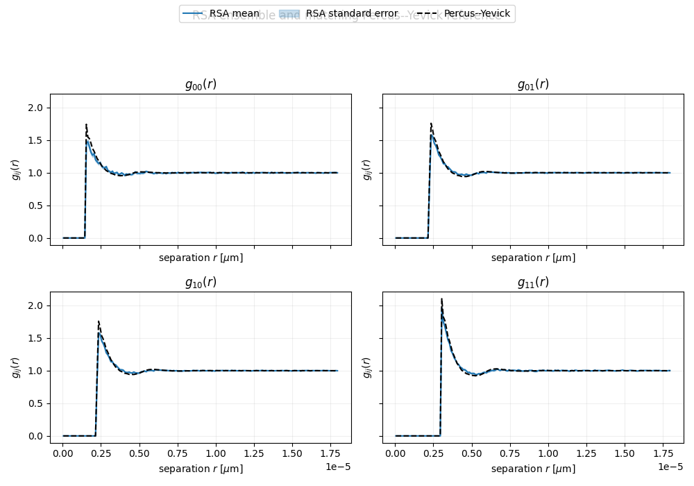
This validation example compares partial pair correlations \(g_{ij}(r)\) from an ensemble of explicit random sequential adsorption (RSA) configurations with a Percus–Yevick hard-sphere-mixture reference at the same radius distribution and volume fraction.

The shaded region is one standard error of the RSA ensemble mean. It shows the finite-ensemble uncertainty; it is not an error band for Percus–Yevick. RSA is irreversible and history-dependent, whereas Percus–Yevick is an analytical equilibrium reference. The curves therefore need not coincide.

import matplotlib.pyplot as plt

from PackLab import analytical, monte_carlo, samplers, ureg

Match the physical mixture in both workflows

radii = [0.75, 1.5] * ureg.micrometer
number_fractions = [0.5, 0.5]
volume_fraction = 0.25

domain = monte_carlo.PackingDomain(
    36.0 * ureg.micrometer,
    36.0 * ureg.micrometer,
    36.0 * ureg.micrometer,
    use_periodic_boundaries=True,
)
sampler = samplers.DiscreteRadiusSampler(radii=radii, weights=number_fractions)

options = monte_carlo.RSAOptions()
options.random_seed = 2026
options.maximum_attempts = 2_050_000
options.maximum_consecutive_rejections = 500_000
options.target_packing_fraction = volume_fraction
options.enforce_radii_distribution = True

estimator = monte_carlo.PackingEstimator(domain, sampler, options, number_of_bins=180)
estimate = estimator.estimate(number_of_samples=60, progress=True)

particle_radii, fractions = sampler.to_bins()
py_domain = analytical.PercusYevickDomain(
    size=100_000 * ureg.micrometer,
    radii=particle_radii,
    volume_fraction=volume_fraction,
    number_fractions=fractions,
)
py_result = analytical.PercusYevickSolver(
    densities=py_domain.particle_densities_per_radius,
    radii=py_domain.radii,
    wavenumber="auto",
).compute(estimate.centers)

PackingEstimator progress
      sample    accepted   attempted  acceptance rate  packing fraction
        1/60        1468       19320           7.598%          0.250209
        2/60        1461       17777           8.218%          0.250209
        3/60        1480       17774           8.327%          0.250134
        4/60        1490       19136           7.786%          0.250247
        5/60        1438       17557           8.190%          0.250134
        6/60        1512       20056           7.539%          0.250285
        7/60        1453       18562           7.828%          0.250171
        8/60        1428       19130           7.465%          0.250020
        9/60        1421       19605           7.248%          0.250020
       10/60        1455       18589           7.827%          0.250247
       11/60        1512       20301           7.448%          0.250020
       12/60        1454       17415           8.349%          0.250209
       13/60        1495       20658           7.237%          0.250171
       14/60        1465       16432           8.916%          0.250096
       15/60        1540       22655           6.798%          0.250285
       16/60        1494       17142           8.715%          0.250134
       17/60        1443       19153           7.534%          0.250058
       18/60        1471       18824           7.814%          0.250058
       19/60        1472       17955           8.198%          0.250096
       20/60        1457       18512           7.871%          0.250058
       21/60        1518       22274           6.815%          0.250247
       22/60        1414       15525           9.108%          0.250020
       23/60        1443       17441           8.274%          0.250058
       24/60        1449       17842           8.121%          0.250020
       25/60        1452       17639           8.232%          0.250134
       26/60        1413       17012           8.306%          0.250247
       27/60        1435       18960           7.569%          0.250020
       28/60        1443       18200           7.929%          0.250058
       29/60        1449       17439           8.309%          0.250020
       30/60        1505       18516           8.128%          0.250020
       31/60        1455       18715           7.775%          0.250247
       32/60        1404       15421           9.104%          0.250171
       33/60        1443       16267           8.871%          0.250058
       34/60        1467       17329           8.466%          0.250171
       35/60        1462       18761           7.793%          0.250247
       36/60        1465       17652           8.299%          0.250096
       37/60        1393       17613           7.909%          0.250020
       38/60        1498       22195           6.749%          0.250285
       39/60        1494       18233           8.194%          0.250134
       40/60        1474       15610           9.443%          0.250171
       41/60        1469       17374           8.455%          0.250247
       42/60        1462       17887           8.174%          0.250247
       43/60        1442       16441           8.771%          0.250020
       44/60        1449       20020           7.238%          0.250285
       45/60        1493       19685           7.584%          0.250096
       46/60        1462       19361           7.551%          0.250247
       47/60        1451       20834           6.965%          0.250096
       48/60        1435       17530           8.186%          0.250285
       49/60        1415       18648           7.588%          0.250058
       50/60        1497       21300           7.028%          0.250247
       51/60        1519       20815           7.298%          0.250020
       52/60        1475       16158           9.129%          0.250209
       53/60        1540       24059           6.401%          0.250020
       54/60        1470       19234           7.643%          0.250020
       55/60        1428       17602           8.113%          0.250020
       56/60        1475       20995           7.025%          0.250209
       57/60        1418       19186           7.391%          0.250171
       58/60        1468       17048           8.611%          0.250209
       59/60        1519       19248           7.892%          0.250020
       60/60        1506       17892           8.417%          0.250058

Compare every partial correlation

The analytical curve is evaluated at the RSA bin centres. A visible difference is therefore due to the models or finite RSA sampling, rather than plotting two different radial grids.

figure, axes = plt.subplots(2, 2, figsize=(10, 7), sharex=True, sharey=True)
standard_error = estimate.std_g / estimator.statistics.completed_samples**0.5

for i, j in ((0, 0), (0, 1), (1, 0), (1, 1)):
    axis = axes[i, j]
    _ = axis.plot(estimate.centers, estimate.mean_g[i, j], color="C0", label="RSA mean")
    _ = axis.fill_between(
        estimate.centers,
        estimate.mean_g[i, j] - standard_error[i, j],
        estimate.mean_g[i, j] + standard_error[i, j],
        color="C0",
        alpha=0.25,
        label="RSA standard error",
    )
    _ = axis.plot(estimate.centers, py_result.g[i, j], "k--", label="Percus--Yevick")
    axis.set_title(rf"$g_{{{i}{j}}}(r)$")
    axis.set_xlabel("separation $r$ [$\\mu$m]")
    axis.set_ylabel(r"$g_{ij}(r)$")
    axis.grid(alpha=0.2)

handles, labels = axes[0, 0].get_legend_handles_labels()
_ = figure.legend(handles, labels, loc="upper center", ncol=3)
figure.suptitle("RSA ensemble and matching Percus--Yevick reference", y=0.98)
figure.tight_layout(rect=(0, 0, 1, 0.91))
plt.show()