Metropolis hard-sphere samples versus Percus–Yevick

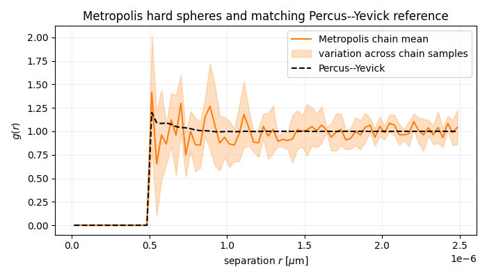
This example compares the pair correlation of fixed-volume hard spheres sampled with Metropolis moves against a Percus–Yevick reference at the same radius and measured volume fraction. RSA is used only to provide a convenient non-overlapping starting configuration; it is not the distribution being compared after the burn-in.

The short chain here is deliberately lightweight for documentation. It shows the workflow, not a production-quality convergence study: assess stationarity, autocorrelation, finite-size effects, and uncertainty before interpreting a scientific comparison.

import matplotlib.pyplot as plt
import numpy as np

from PackLab import analytical, monte_carlo, samplers, ureg

Construct a fixed-volume hard-sphere system

radii = np.array([0.25]) * ureg.micrometer
radius = radii[0]
domain = monte_carlo.PackingDomain(
    5.0 * ureg.micrometer,
    5.0 * ureg.micrometer,
    5.0 * ureg.micrometer,
    use_periodic_boundaries=True,
)

rsa_options = monte_carlo.RSAOptions()
rsa_options.random_seed = 2026
rsa_options.maximum_attempts = 100_000
rsa_options.target_packing_fraction = 0.05
initial_result = monte_carlo.RSASimulator(
    domain,
    samplers.ConstantRadiusSampler(radius, bins=1),
    rsa_options,
).run()

metropolis_options = monte_carlo.MetropolisOptions()
metropolis_options.random_seed = 2027
metropolis_options.maximum_displacement = 0.05 * ureg.micrometer
metropolis_options.number_of_sweeps = 100  # burn-in for this small demonstration
simulator = monte_carlo.MetropolisSimulator(
    domain,
    initial_result.sphere_configuration,
    metropolis_options,
)
simulator.run()

<PackLab.monte_carlo.results.PackingResult object at 0x7f91a3569fd0>

Sample the Metropolis chain and calculate the reference

sample_curves = []
for _ in range(5):
    # Consecutive samples remain correlated; production calculations should
    # choose this interval from an autocorrelation analysis.
    metropolis_options.number_of_sweeps = 40
    sample = simulator.run()
    centers, partial_g = sample.compute_partial_pair_correlation_function(
        n_bins=80,
        maximum_pairs=100_000,
    )
    sample_curves.append(partial_g[0, 0])

mean_g = np.mean(sample_curves, axis=0)
sample_spread = np.std(sample_curves, axis=0, ddof=1)
volume_fraction = initial_result.statistics.packing_fraction_geometry

py_domain = analytical.PercusYevickDomain(
    size=100_000 * ureg.micrometer,
    radii=radii,
    volume_fraction=volume_fraction,
    number_fractions=[1.0],
)
py_result = analytical.PercusYevickSolver(
    densities=py_domain.particle_densities_per_radius,
    radii=py_domain.radii,
    wavenumber="auto",
).compute(centers)

print(f"Metropolis acceptance rate: {simulator.statistics.acceptance_rate:.3f}")
print(f"Measured volume fraction: {volume_fraction:.3f}")

Metropolis acceptance rate: 0.970
Measured volume fraction: 0.050

Plot the comparison

figure, axis = plt.subplots(figsize=(7, 4))
_ = axis.plot(centers, mean_g, color="C1", label="Metropolis chain mean")
_ = axis.fill_between(
    centers,
    mean_g - sample_spread,
    mean_g + sample_spread,
    color="C1",
    alpha=0.25,
    label="variation across chain samples",
)
_ = axis.plot(centers, py_result.g[0, 0], "k--", label="Percus--Yevick")
axis.set_xlabel("separation $r$ [$\\mu$m]")
axis.set_ylabel("$g(r)$")
axis.set_title("Metropolis hard spheres and matching Percus--Yevick reference")
axis.grid(alpha=0.2)
_ = axis.legend()
figure.tight_layout()
plt.show()