PackLab Percus–Yevick versus the Tsang et al. reference

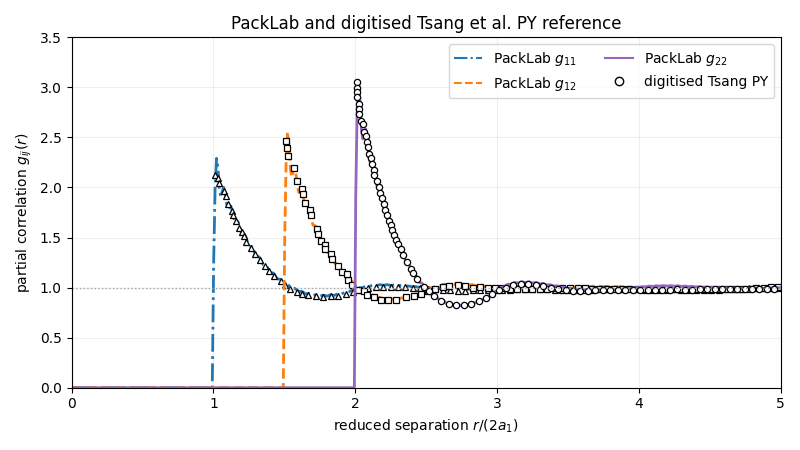
This validation example compares PackLab’s Percus–Yevick (PY) solution for a binary hard-sphere mixture with manually digitised PY curves from Figure 8.3.4 of Tsang, Kong, Ding, and Ao (2001). The book uses radii \(a_2 = 2a_1\), partial volume fractions \(f_1=0.2\) and \(f_2=0.1\), and reduced separation \(r/(2a_1)\).

The digitised values originate from a printed figure, rather than the source numerical data, so this is a visual reference comparison rather than a high-precision error benchmark.

import os
from pathlib import Path

import matplotlib.pyplot as plt
from matplotlib.lines import Line2D
import numpy as np

from PackLab import analytical, ureg

Load the digitised reference data

if "PACKLAB_DOCS_ROOT" in os.environ:
    docs_root = Path(os.environ["PACKLAB_DOCS_ROOT"])
else:
    docs_root = Path(__file__).resolve().parents[2]
data_path = (
    docs_root
    / "manuscript"
    / "softwareX"
    / "data"
    / "tsang_2001_figure_8_3_4_digitized.csv"
)
digitized = np.genfromtxt(data_path, delimiter=",", names=True, dtype=None, encoding="utf-8")

Match the mixture and calculate PackLab’s PY solution

radii = np.array([1.0, 2.0]) * ureg.micrometer
partial_volume_fractions = np.array([0.2, 0.1])

# The book reports partial *volume* fractions. Convert them to the number
# fractions required by the mixture solver, n_i proportional to f_i/a_i^3.
number_fractions = partial_volume_fractions / radii.to("micrometer").magnitude**3
number_fractions /= number_fractions.sum()

domain = analytical.PercusYevickDomain(
    size=100_000 * ureg.micrometer,
    radii=radii,
    volume_fraction=partial_volume_fractions.sum(),
    number_fractions=number_fractions,
)
reduced_separation = np.linspace(0.0, 5.0, 500)
result = analytical.PercusYevickSolver(
    densities=domain.particle_densities_per_radius,
    radii=domain.radii,
    wavenumber="auto",
).compute(reduced_separation * 2.0 * radii[0])

Compare all three partial correlations

figure, axis = plt.subplots(figsize=(8, 4.5))
curves = (
    (r"$g_{11}$", "g11", (0, 0), "C0", "-.", "^"),
    (r"$g_{12}$", "g12", (0, 1), "C1", "--", "s"),
    (r"$g_{22}$", "g22", (1, 1), "C4", "-", "o"),
)

for label, component_pair, indices, colour, line_style, marker in curves:
    _ = axis.plot(
        reduced_separation,
        result.g[indices],
        color=colour,
        linestyle=line_style,
        linewidth=2,
    )
    reference = digitized[digitized["component_pair"] == component_pair]
    _ = axis.plot(
        reference["reduced_separation"],
        reference["g_ij"],
        linestyle="none",
        marker=marker,
        markersize=4.5,
        markerfacecolor="white",
        markeredgecolor="black",
        markeredgewidth=0.9,
    )

_ = axis.axhline(1.0, color="0.65", linestyle=":", linewidth=1)
_ = axis.set(
    xlim=(0.0, 5.0),
    ylim=(0.0, 3.5),
    xlabel=r"reduced separation $r/(2a_1)$",
    ylabel=r"partial correlation $g_{ij}(r)$",
    title="PackLab and digitised Tsang et al. PY reference",
)
axis.grid(alpha=0.2)
_ = axis.legend(
    handles=[
        Line2D([], [], color=colour, linestyle=line_style, label=f"PackLab {label}")
        for label, _, _, colour, line_style, _ in curves
    ]
    + [
        Line2D(
            [], [], color="black", linestyle="none", marker="o", markerfacecolor="white",
            label="digitised Tsang PY",
        )
    ],
    ncol=2,
)
figure.tight_layout()
plt.show()