

Note
Go to the end to download the full example code.
Explore a synthetic objective landscape#
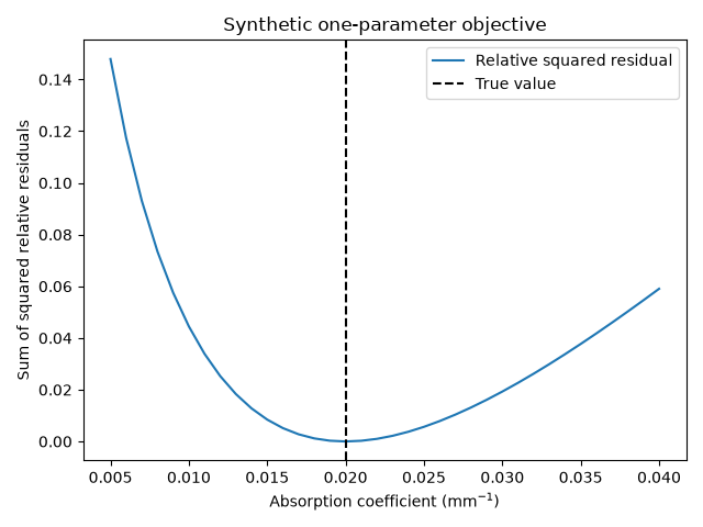
Compare candidate absorption coefficients with noiseless fluence values from an infinite-medium P1 calculation. The true and candidate data use the same model; this illustrates an objective function, not recovery accuracy for a real sensor. All values are illustrative.
import matplotlib.pyplot as plt
import numpy as np
import MomentRT

ureg = MomentRT.ureg
Set up the forward calculation#
The Cartesian mesh is an observation window, not a physical boundary. An even number of points keeps the ideal point-source singularity off the grid. The source power, scattering and all other parameters are treated as known.
mesh = MomentRT.CartesianMesh(
    shape=(20, 20, 20),
    spacing=np.full(3, 0.4) * ureg.mm,
    origin=np.full(3, -3.8) * ureg.mm,
)
source = MomentRT.PointSource(
    position=np.zeros(3) * ureg.mm,
    wavelength=850 * ureg.nm,
    optical_power=1 * ureg.mW,
)
solver = MomentRT.InfiniteP1()
Generate synthetic observations#
Sample two nodal fluence values, not detector powers. The observations and predictions share this exact forward model; no noise or uncertainty is added.
true_absorption = 0.02
sample_indices = ((12, 10, 10), (16, 10, 10))


def calculate_fluence(*, absorption_per_mm: float) -> MomentRT.SimulationResult:
    """Calculate the field at a specified absorption in inverse millimeters.

    Parameters
    ----------
    absorption_per_mm : float
        Absorption coefficient in inverse millimeters.

    Returns
    -------
    SimulationResult
        Infinite-medium fluence sampled on the observation grid.
    """
    material = MomentRT.Material(
        absorption=absorption_per_mm / ureg.mm,
        reduced_scattering=1 / ureg.mm,
        refractive_index=1.4,
        phase_function=MomentRT.Isotropic(),
    )
    simulation = MomentRT.Simulation(
        medium=MomentRT.HomogeneousMedium(material=material),
        source=source,
        mesh=mesh,
        solver=solver,
    )
    return simulation.run()


observed_result = calculate_fluence(absorption_per_mm=true_absorption)
observed_field = observed_result.fluence.values.to("W/m^2").magnitude
observations = np.array([observed_field[index] for index in sample_indices])
Evaluate the mismatch#
Sum squared relative residuals so the two observations have equal relative weight. This weighting is illustrative and is not a measurement noise model. A minimum at the true value is expected because both sides use the same model.
candidates = np.linspace(0.005, 0.04, 36)
objective = []
for candidate in candidates:
    result = calculate_fluence(absorption_per_mm=float(candidate))
    field = result.fluence.values.to("W/m^2").magnitude
    predictions = np.array([field[index] for index in sample_indices])
    objective.append(np.sum(((predictions - observations) / observations) ** 2))

figure, axes = plt.subplots()
axes.plot(candidates, objective, label="Relative squared residual")
axes.axvline(true_absorption, color="black", linestyle="--", label="True value")
axes.set_xlabel("Absorption coefficient (mm$^{-1}$)")
axes.set_ylabel("Sum of squared relative residuals")
axes.set_title("Synthetic one-parameter objective")
axes.legend()
figure.tight_layout()
Inspect the synthetic fluence field#
This field belongs to the true absorption. The box is only an observation window; the example does not model contact detectors or finite boundaries. A well-defined minimum here does not establish identifiability with noise, unknown nuisance parameters, different models, or experimental data.
gallery_system_figure = observed_result.fluence.plot(
    view="volume",
    scale="log",
    overlays=[source],
    show=False,
)
gallery_system_figure.update_layout(title="Infinite-medium fluence: observation window")
Total running time of the script: (0 minutes 0.201 seconds)