

Note
Go to the end to download the full example code.
Compare P1 and SP3 with independent planar slab references#
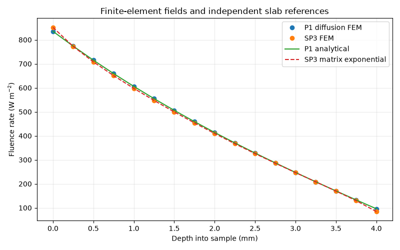
Compare finite-element centerline fluence against two independent 1D solutions: a closed-form P1 diffusion slab and a matrix-exponential SP3 slab. These references check implementation and spatial discretization for this planar setup; they do not establish accuracy against radiative transfer or validate either model for a sensor geometry.
import os
import matplotlib.pyplot as plt
import numpy as np
from scipy.linalg import expm
import MomentRT

ureg = MomentRT.ureg
show_figures = os.environ.get("MOMENTRT_SPHINX_GALLERY") != "1"
Configure a laterally uniform slab#
Reflecting side faces preserve a one-dimensional solution. Both models use the same homogeneous material, diffuse illumination, mesh, and matched-index top and bottom faces.
absorption = 20 / ureg.meter
reduced_scattering = 1000 / ureg.meter
anisotropy = 0.7
thickness = 4 * ureg.millimeter

material = MomentRT.Material(
    absorption=absorption,
    reduced_scattering=reduced_scattering,
    refractive_index=1.4,
    anisotropy=anisotropy,
    phase_function=MomentRT.phase_function.HenyeyGreenstein(),
)

sample = MomentRT.StructuredMedium(
    origin=np.zeros(3) * ureg.millimeter,
    size=np.array([2, 2, 4]) * ureg.millimeter,
)
sample.add_background(material=material)

mesh = MomentRT.CartesianMesh.from_sample(sample=sample, shape=(5, 5, 17))
source = MomentRT.UniformSurfaceSource(
    face="z_min",
    wavelength=970 * ureg.nanometer,
    optical_power=1 * ureg.milliwatt,
)
open_face = MomentRT.RobinBoundary(effective_reflectance=0)
boundaries = {face: MomentRT.ReflectingBoundary() for face in MomentRT.boundary.FACES}
boundaries["z_min"] = open_face
boundaries["z_max"] = open_face

simulations = {
    "P1 diffusion": MomentRT.Simulation(
        medium=sample,
        source=source,
        mesh=mesh,
        solver=MomentRT.P1(boundaries=boundaries),
    ),
    "SP3": MomentRT.Simulation(
        medium=sample,
        source=source,
        mesh=mesh,
        solver=MomentRT.SP3(boundaries=boundaries),
    ),
}

depth = mesh.points[0, 0, :, 2].to("meter").magnitude
length = thickness.to("meter").magnitude
mu_a = absorption.to("1/meter").magnitude
mu_s1 = reduced_scattering.to("1/meter").magnitude
incident = source.optical_power.to("watt").magnitude / np.prod(
    sample.size[:2].to("meter").magnitude
)
Calculate an independent closed-form P1 solution#
The homogeneous diffusion equation has hyperbolic solutions. Solve its two boundary equations directly, independently of the FEM matrix assembly.
diffusion_coefficient = 1 / (3 * (mu_a + mu_s1))
attenuation = np.sqrt(mu_a / diffusion_coefficient)
beta = open_face.leakage_coefficient
source_coefficient = 2 / (1 + open_face.effective_reflectance)
top_row = np.array([beta, -diffusion_coefficient * attenuation])
bottom_row = np.array(
    [
        diffusion_coefficient * attenuation * np.sinh(attenuation * length)
        + beta * np.cosh(attenuation * length),
        diffusion_coefficient * attenuation * np.cosh(attenuation * length)
        + beta * np.sinh(attenuation * length),
    ]
)
constants = np.linalg.solve(
    np.vstack((top_row, bottom_row)),
    np.array([source_coefficient * incident, 0]),
)
p1_reference = constants[0] * np.cosh(attenuation * depth) + constants[1] * np.sinh(
    attenuation * depth
)
Calculate an independent SP3 matrix-exponential solution#
Integrate the first-order moment system through the slab and solve its Marshak conditions at both ends. This analytic 1D reference is independent of MomentRT’s three-dimensional finite-element assembly.
mu_1 = mu_a + mu_s1
mu_2 = mu_a + mu_s1 * (1 + anisotropy)
mu_3 = mu_a + mu_s1 * (1 + anisotropy + anisotropy**2)
generator = np.array(
    [
        [0, 0, -3 * mu_1, 0],
        [0, 0, 0, -7 * mu_3],
        [-mu_a, 2 * mu_a / 3, 0, 0],
        [2 * mu_a / 3, -(4 * mu_a + 5 * mu_2) / 9, 0, 0],
    ]
)
transfer = expm(generator * length)
top = np.array([[0.5, -0.125, 1, 0], [-0.125, 7 / 24, 0, 1]])
bottom = np.array([[-0.5, 0.125, 1, 0], [0.125, -7 / 24, 0, 1]])
initial = np.linalg.solve(
    np.vstack((top, bottom @ transfer)),
    np.array([2 * incident, -incident / 2, 0, 0]),
)
states = np.array([expm(generator * position) @ initial for position in depth])
sp3_reference = states[:, 0] - 2 * states[:, 1] / 3
Compare FEM fields with the references#
The curves should approach their corresponding references as the mesh is refined. P1 and SP3 are different transport approximations, so their analytical references are distinct even when the numerical mesh is shared.
figure, axes = plt.subplots(figsize=(8, 5))
for label, simulation in simulations.items():
    report = simulation.validate()
    print(f"{label} configuration:\n{report.summary()}")
    result = simulation.run()
    actual = result.fluence.values[2, 2, :].to("watt / meter**2").magnitude
    reference = p1_reference if label == "P1 diffusion" else sp3_reference
    relative_error = np.linalg.norm(actual - reference) / np.linalg.norm(reference)
    print(f"{label} relative L2 error against its slab reference: {relative_error:.3%}")
    axes.plot(depth * 1e3, actual, "o", label=f"{label} FEM")
axes.plot(depth * 1e3, p1_reference, label="P1 analytical")
axes.plot(depth * 1e3, sp3_reference, "--", label="SP3 matrix exponential")
axes.set_xlabel("Depth into sample (mm)")
axes.set_ylabel("Fluence rate (W m$^{-2}$)")
axes.set_title("Finite-element fields and independent slab references")
axes.grid(True, alpha=0.25)
axes.legend()
figure.tight_layout()
plt.show() if show_figures else None
P1 diffusion configuration:
Configuration valid
Warning: Footprint sampling alone does not establish mesh convergence or transport accuracy.
Model note: Diffusion is a steady-state P1 approximation on a finite sample, using linear tetrahedra and centroid-sampled material coefficients.
Model note: Fluence is continuous across internal interfaces; refractive-index jumps are unsupported, while absorption and reduced scattering may vary.
Model note: P1 diffusion is least reliable close to illumination and in weakly scattering regions; mesh refinement does not remove this model error.
Model note: Robin effective_reflectance is supplied explicitly and is not inferred from refractive index.
Source sampled area: 4×10⁻⁶ m²
P1 diffusion relative L2 error against its slab reference: 0.004%
SP3 configuration:
Configuration valid
Warning: Footprint sampling alone does not establish mesh convergence or transport accuracy.
Model note: SP3 is a steady-state simplified P3 angular-moment approximation; it uses each material's normalized phase-function moments through degree 3.
Model note: SP3 assumes isotropic incoming diffuse radiance, requires zero-reflectance Robin conditions on illuminated faces, permits reflecting unilluminated faces, and requires equal internal refractive indices.
Model note: SP3 agreement with a slab reference verifies this implementation for that case, not accuracy for arbitrary geometries or sensors.
Model note: Detector angular acceptance uses a separate Lambertian approximation.
Source sampled area: 4×10⁻⁶ m²
SP3 relative L2 error against its slab reference: 0.044%
Total running time of the script: (0 minutes 0.227 seconds)