

Note
Go to the end to download the full example code.
Uniform illumination on a sample face#
Illuminate an entire finite sample face with a uniform diffuse partial current, solve the P1 finite-element model, and inspect the three-dimensional fluence field. The input power is already coupled into the sample.
import matplotlib.pyplot as plt
import numpy as np
import MomentRT
from MomentRT import (
    P1,
    Material,
    RobinBoundary,
    Simulation,
    StructuredMedium,
    TetrahedralMesh,
    UniformSurfaceSource,
    ureg,
)
Create the homogeneous slab#
Set all optical properties and dimensions explicitly for this wavelength.
material = Material(
    phase_function=MomentRT.phase_function.HenyeyGreenstein(),
    absorption=0.03 / ureg.millimeter,
    reduced_scattering=1.0 / ureg.millimeter,
    refractive_index=1.4,
)

sample = StructuredMedium(
    origin=(-4, -4, 0) * ureg.millimeter,
    size=(8, 8, 4) * ureg.millimeter,
)

sample.add_background(
    material=material,
)
Configure the mesh, source, and six faces#
The incoming diffuse power is spread uniformly across the complete z_min face. All faces use the same explicit effective diffuse reflectance.
mesh = TetrahedralMesh.from_sample(
    sample=sample,
    resolution=0.7 * ureg.millimeter,
)

source = UniformSurfaceSource(
    face="z_min",
    wavelength=970 * ureg.nanometer,
    optical_power=1 * ureg.milliwatt,
)

boundary = RobinBoundary(
    effective_reflectance=0.5,
)

solver = P1(
    boundaries=MomentRT.Boundaries.uniform(condition=boundary),
)
Solve and view the field#
The 3D plot is made from the nodal finite-element fluence values.
simulation = Simulation(
    medium=sample,
    source=source,
    mesh=mesh,
    solver=solver,
)

result = simulation.run()

# The illumination patch is independent of the fluence opacity control.
figure = result.fluence.plot(
    view="volume",
    scale="log",
    display_resolution=0.4 * ureg.millimeter,
    overlays=[source],
    show=False,
)
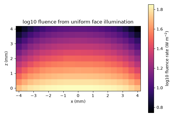
Preview a central plane#
A static section uses the same interpolated display grid as the volume.
display_field = result.fluence.resample(resolution=0.4 * ureg.millimeter)

display_mesh = display_field.mesh

fluence_values = display_field.values.to("watt / meter**2").magnitude

center_y = display_mesh.shape[1] // 2

x_axis = (
    (
        display_mesh.origin[0]
        + np.arange(display_mesh.shape[0]) * display_mesh.spacing[0]
    )
    .to("millimeter")
    .magnitude
)

z_axis = (
    (
        display_mesh.origin[2]
        + np.arange(display_mesh.shape[2]) * display_mesh.spacing[2]
    )
    .to("millimeter")
    .magnitude
)

figure_static, axes = plt.subplots(figsize=(6, 4))

image = axes.pcolormesh(
    x_axis,
    z_axis,
    np.log10(fluence_values[:, center_y, :].T),
    shading="auto",
    cmap="magma",
)

axes.set_aspect("equal")
axes.set_xlabel("x (mm)")
axes.set_ylabel("z (mm)")
axes.set_title("log10 fluence from uniform face illumination")
figure_static.colorbar(image, ax=axes, label="log10 fluence rate (W m$^{-2}$)")
figure_static.tight_layout()


print(f"Incoming power: {result.energy_balance['incoming_power']}")
print(f"Absorbed power: {result.energy_balance['absorbed_power']}")
print(f"Escaping power: {result.energy_balance['escaping_power']}")
Incoming power: 1 milliwatt
Absorbed power: 0.00020510637958009797 watt
Escaping power: 0.000794893620419902 watt
Inspect the modeled geometry#
This view shows the configured geometry and instrument footprints.
gallery_system_figure = simulation.plot_system(show=False)
Total running time of the script: (0 minutes 0.583 seconds)