

Note
Go to the end to download the full example code.
Follow a diffuse pulse through layered tissue#
Solve the time-dependent P1 fluence and current equations for an illustrative layered sample and a diffuse contact source. The result includes a detector power trace and a fluence snapshot. This example demonstrates the workflow; it does not establish mesh convergence or early-time transport accuracy.
import matplotlib.pyplot as plt
import numpy as np
import MomentRT

ureg = MomentRT.ureg
Configure tissue and contacts#
Both materials use the same refractive index. The optical coefficients and uniform energy speed are illustrative; the speed is specified independently and is not inferred from the refractive index.
background = MomentRT.material.Material(
    absorption=0.02 / ureg.mm,
    reduced_scattering=1 / ureg.mm,
    refractive_index=1.4,
    phase_function=MomentRT.phase_function.Isotropic(),
)
upper = MomentRT.material.Material(
    absorption=0.04 / ureg.mm,
    reduced_scattering=1.5 / ureg.mm,
    refractive_index=1.4,
    phase_function=MomentRT.phase_function.Isotropic(),
)
sample = MomentRT.medium.StructuredMedium(
    origin=(-2, -2, 0) * ureg.mm,
    size=(4, 4, 3) * ureg.mm,
)
sample.add_background(material=background)
sample.add_layer(
    name="Upper layer",
    thickness=1 * ureg.mm,
    material=upper,
)
source = MomentRT.source.SurfaceSource.on_face(
    sample=sample,
    face="z_min",
    coordinates=(-0.8, 0) * ureg.mm,
    radius=0.7 * ureg.mm,
    wavelength=850 * ureg.nm,
    optical_power=1 * ureg.mW,
)
detector = MomentRT.detector.SurfaceDetector.full_hemisphere_on_face(
    sample=sample,
    face="z_min",
    coordinates=(0.8, 0) * ureg.mm,
    radius=0.7 * ureg.mm,
)
mesh = MomentRT.mesh.TetrahedralMesh.from_sample(
    sample=sample,
    resolution=0.7 * ureg.mm,
)
mesh.refine_near(
    objects=[source, detector],
    resolution=0.35 * ureg.mm,
    distance=0.3 * ureg.mm,
)
Specify and solve the pulse#
The dimensionless profile multiplies the source’s coupled optical power. It starts at zero, matching zero initial fluence and current, and is interpolated linearly between the explicit time samples. Robin reflectance is an explicit diffuse partial-current coefficient.
times = np.linspace(0, 120, 121) * ureg.ps
pulse_time = times.to("ps").magnitude / 15
profile = pulse_time * np.exp(1 - pulse_time)
solver = MomentRT.transport.TransientP1(
    boundaries=MomentRT.boundary.Boundaries.uniform(
        condition=MomentRT.boundary.RobinBoundary(effective_reflectance=0),
    ),
    times=times,
    power_profile=profile,
    energy_speed=2e8 * ureg.m / ureg.s,
)
simulation = MomentRT.simulation.Simulation(
    medium=sample,
    source=source,
    mesh=mesh,
    solver=solver,
    detectors={"contact": detector},
)
result = simulation.run()
Inspect the detector trace and conservation#
The detector integrates boundary irradiance using a Lambertian angular model; it does not resolve external optics. Negative values are preserved. Interval energy residuals use the midpoint rule and are only a conservation diagnostic.
figure, axes = plt.subplots(1, 2, figsize=(10, 4), constrained_layout=True)
axes[0].plot(
    result.times.to("ps").magnitude,
    result.incoming_power.to("mW").magnitude,
    label="Incoming",
)
axes[0].plot(
    result.times.to("ps").magnitude,
    result.detector_power["contact"].to("mW").magnitude,
    label="Collected",
)
axes[0].set_xlabel("Time (ps)")
axes[0].set_ylabel("Power (mW)")
axes[0].legend()
axes[1].plot(result.times.to("ps").magnitude, result.stored_energy.to("pJ").magnitude)
axes[1].set_xlabel("Time (ps)")
axes[1].set_ylabel("Stored energy (pJ)")
print(
    f"Maximum midpoint energy residual: {np.max(np.abs(result.interval_energy_residual)).to('W'):~P}"
)
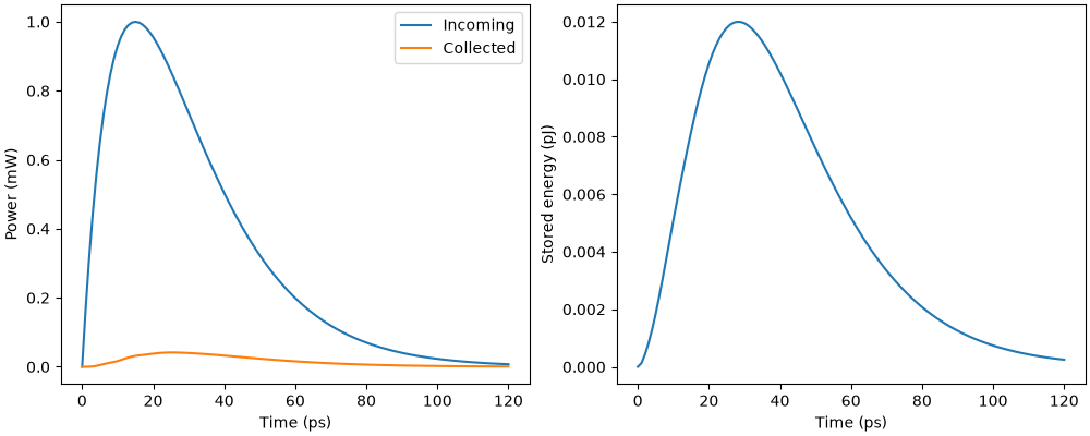
Maximum midpoint energy residual: 2.3310346708438345×10⁻¹⁸ W
View fluence at the pulse peak#
Tetrahedral nodal fluence is interpolated to a display grid. The physical time-dependent current remains element-centered and is not smoothed. Refine the spatial and temporal grids independently and compare against a transport reference before interpreting early-time or near-source predictions.
peak_index = int(np.argmax(profile))
peak = result.frames[peak_index]
gallery_system_figure = peak.fluence.plot(
    view="volume",
    scale="linear",
    display_resolution=0.3 * ureg.mm,
    overlays=[source, detector],
    show=False,
)
gallery_system_figure.update_layout(
    title=f"Transient P1 fluence at {times[peak_index]:~P}"
)
Total running time of the script: (0 minutes 1.107 seconds)