

Note
Go to the end to download the full example code.
Build analytical source spectra#
Create Gaussian and Lorentzian wavelength spectra, compare their shapes, then use one with an embedded point source. These are illustrative profiles, not measured LED spectra. Both are normalized to the same power over the explicit finite wavelength interval.
import matplotlib.pyplot as plt
import numpy as np
import MomentRT
from MomentRT.models.spectrum import Gaussian, Lorentzian

ureg = MomentRT.ureg
Choose the wavelength grid and line widths#
Full width at half maximum is measured in wavelength, not frequency. The finite interval truncates both profiles; the longer Lorentzian tails make its choice especially important. Each trapezoidal integral over this grid is normalized to the stated optical power.
wavelengths = np.linspace(750, 950, 81) * ureg.nm
parameters = {
    "wavelengths": wavelengths,
    "center": 850 * ureg.nm,
    "fwhm": 30 * ureg.nm,
    "optical_power": 1 * ureg.mW,
}
gaussian = Gaussian(**parameters)
lorentzian = Lorentzian(**parameters)
print(f"Gaussian integrated power: {gaussian.optical_power.to('mW'):~P}")
print(f"Lorentzian integrated power: {lorentzian.optical_power.to('mW'):~P}")

figure, axes = plt.subplots()
for name, spectrum in (("Gaussian", gaussian), ("Lorentzian", lorentzian)):
    axes.plot(
        spectrum.wavelengths.to("nm").magnitude,
        spectrum.spectral_power.to("uW/nm").magnitude,
        label=name,
    )
axes.set_xlabel("Vacuum wavelength (nm)")
axes.set_ylabel("Spectral power (µW/nm)")
axes.legend()
figure.tight_layout()
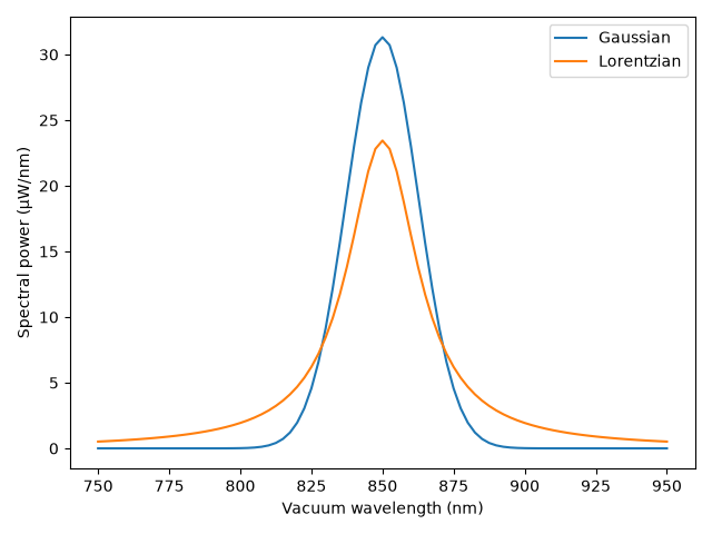
Gaussian integrated power: 1.0 mW
Lorentzian integrated power: 1.0 mW
Attach a spectrum to a source#
Source geometry and emission are independent: swap the spectrum for the
Lorentzian above without changing the source position or medium. run
computes monochromatic reference fields across the source grid. For a real
broadband calculation, also check spectral resolution and material coverage.
source = MomentRT.PointSource(
    position=np.zeros(3) * ureg.mm,
    spectrum=gaussian,
)
material = MomentRT.Material(
    absorption=0.02 / ureg.mm,
    reduced_scattering=1 / ureg.mm,
    refractive_index=1.4,
    phase_function=MomentRT.Isotropic(),
)
mesh = MomentRT.CartesianMesh(
    shape=(20, 20, 20),
    spacing=np.full(3, 0.4) * ureg.mm,
    origin=np.full(3, -3.8) * ureg.mm,
)
simulation = MomentRT.Simulation(
    medium=MomentRT.HomogeneousMedium(material=material),
    source=source,
    mesh=mesh,
    solver=MomentRT.InfiniteP1(),
)
result = simulation.run()
Inspect a reference fluence field#
The central-wavelength reference field uses the result’s stated reference power, not the integrated broadband source power or a spectral density. The volume is an observation window in an infinite medium, not a sample boundary.
reference = result.reference_results.results[len(wavelengths) // 2]
print(f"Reference power: {result.reference_optical_power:~P}")
gallery_system_figure = reference.fluence.plot(
    view="volume",
    scale="log",
    overlays=[source],
    show=False,
)
gallery_system_figure.update_layout(title="Infinite-medium fluence: observation window")
Reference power: 1 W
Total running time of the script: (0 minutes 0.209 seconds)