Analytical wavenumber-grid cost

Time a fixed binary mixture on increasingly fine manual grids. Grid spacing resolves at least 12 samples per longest-distance oscillation; decreasing the real-space resolution increases the high-wavenumber cutoff. The median of three runs is a timing measure, not an accuracy assessment. Report machine, software versions and thread settings when comparing measurements.

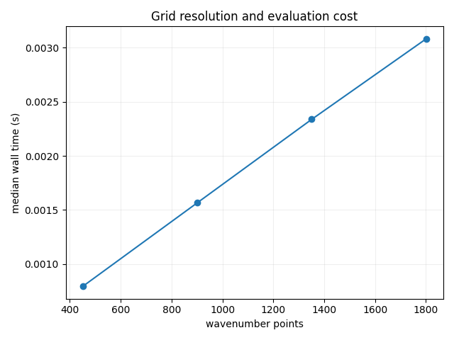
451 wavenumbers: median 0.0008 s
901 wavenumbers: median 0.0016 s
1351 wavenumbers: median 0.0023 s
1801 wavenumbers: median 0.0031 s

from time import perf_counter
import matplotlib.pyplot as plt
import numpy as np
from PackLab import analytical, ureg

radii = np.array([0.1, 0.2]) * ureg.micrometer
domain = analytical.PercusYevickDomain(
    size=100 * ureg.micrometer, radii=radii, volume_fraction=0.2, number_fractions=[0.5, 0.5]
)
distances = np.linspace(0, 1.5, 150) * ureg.micrometer
counts, timings = [], []
for divisor in (5, 10, 15, 20):
    grid = analytical.make_wavenumber_grid(radii.min() / divisor, distances.max(), 12)
    solver = analytical.PercusYevickSolver(
        densities=domain.particle_densities_per_radius, radii=radii, wavenumber=grid
    )
    runs = []
    for _ in range(3):
        start = perf_counter()
        solver.compute(distances)
        runs.append(perf_counter() - start)
    counts.append(len(grid))
    timings.append(np.median(runs))
    print(f"{len(grid)} wavenumbers: median {timings[-1]:.4f} s")
figure, axis = plt.subplots()
axis.plot(counts, timings, "o-")
axis.set(
    xlabel="wavenumber points",
    ylabel="median wall time (s)",
    title="Grid resolution and evaluation cost",
)
axis.grid(alpha=0.2)
figure.tight_layout()