Sphere: Coupling vs numerical aperture

Importing the package dependencies: numpy, PyMieSim

import numpy as np

from PyMieSim import experiment
from PyMieSim import single
from PyMieSim.units import degree, watt, AU, RIU, meter, nanometer
from PyOptik import Material

Defining the source to be employed.

source = experiment.source.Gaussian(
    wavelength=500 * nanometer,
    polarization=0 * degree,
    optical_power=1e-3 * watt,
    NA=0.2 * AU
)

Defining the ranging parameters for the scatterer distribution

scatterer = experiment.scatterer.Sphere(
    diameter=500e-9 * meter,
    property=Material.BK7,
    medium_property=1 * RIU,
    source=source
)

Defining the detector to be employed.

detector = experiment.detector.Photodiode(
    NA=np.linspace(0.1, 1, 150) * AU,
    phi_offset=0 * degree,
    gamma_offset=[0, 10] * degree,
    polarization_filter=None,
    sampling=2000 * AU
)

Defining the experiment setup

setup = experiment.Setup(scatterer=scatterer, source=source, detector=detector)

/opt/hostedtoolcache/Python/3.11.13/x64/lib/python3.11/site-packages/PyOptik/material/base_class.py:60: UserWarning: Wavelength range goes from 500.0 nm to 500.0 nm which is outside the allowable range of 5.0 µm to 33.333 µm µm. [Material: BK7]
  warnings.warn(

Measuring the properties

dataframe = setup.get('coupling', drop_unique_level=True)

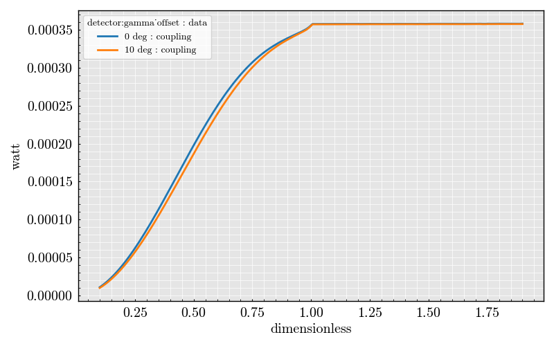
Plotting the results

dataframe.plot(x='detector:NA')

single_source = single.Gaussian(
    wavelength=950 * nanometer,
    polarization=0 * degree,
    optical_power=1e-3 * watt,
    NA=0.2 * AU
)

single_scatterer = single.scatterer.Sphere(
    diameter=500 * nanometer,
    property=Material.BK7,
    medium_property=1 * RIU,
    source=single_source
)


print(single_scatterer.Qsca * 1e-3)

/opt/hostedtoolcache/Python/3.11.13/x64/lib/python3.11/site-packages/PyOptik/material/base_class.py:60: UserWarning: Wavelength range goes from 949.9999999999999 nm to 949.9999999999999 nm which is outside the allowable range of 5.0 µm to 33.333 µm µm. [Material: BK7]
  warnings.warn(
0.00057801149997312