Array-based scattering calculations

This example demonstrates how to compute far fields, S1/S2 amplitudes and Stokes parameters using arbitrary phi and theta arrays.

import numpy as np
from PyMieSim.units import ureg
import matplotlib.pyplot as plt

from PyMieSim.single.scatterer import Sphere
from PyMieSim.single.source import PlaneWave

Create a simple plane wave source

source = PlaneWave(
    wavelength=632.8 * ureg.nanometer,
    polarization=0 * ureg.degree,
    amplitude=1 * ureg.volt / ureg.meter,
)

scatterer = Sphere(
    diameter=200 * ureg.nanometer,
    refractive_index=1.5 * ureg.RIU,
    medium_refractive_index=1.0 * ureg.RIU,
    source=source,
)

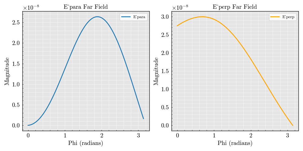
phi = np.linspace(0, np.pi, 150) * ureg.radian
theta = np.linspace(0, np.pi / 2, 150) * ureg.radian

E_para, E_perp = scatterer.get_farfields(phi=phi, theta=theta, distance=1 * ureg.meter)

plt.figure(figsize=(10, 5))
plt.subplot(1, 2, 1)
plt.plot(phi, np.abs(E_para), label="E_para")
plt.title("E_para Far Field")
plt.xlabel("Phi (radians)")
plt.ylabel("Magnitude")
plt.legend()
plt.subplot(1, 2, 2)
plt.plot(phi, np.abs(E_perp), label="E_perp", color="orange")
plt.title("E_perp Far Field")
plt.xlabel("Phi (radians)")
plt.ylabel("Magnitude")
plt.legend()
plt.tight_layout()
plt.show()

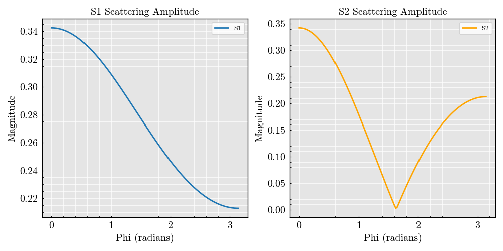
S1 and S2 scattering amplitudes

S1, S2 = scatterer.get_s1s2(phi=phi)

plt.figure(figsize=(10, 5))
plt.subplot(1, 2, 1)
plt.plot(phi, np.abs(S1), label="S1")
plt.title("S1 Scattering Amplitude")
plt.xlabel("Phi (radians)")
plt.ylabel("Magnitude")
plt.legend()
plt.subplot(1, 2, 2)
plt.plot(phi, np.abs(S2), label="S2", color="orange")
plt.title("S2 Scattering Amplitude")
plt.xlabel("Phi (radians)")
plt.ylabel("Magnitude")
plt.legend()
plt.tight_layout()
plt.show()

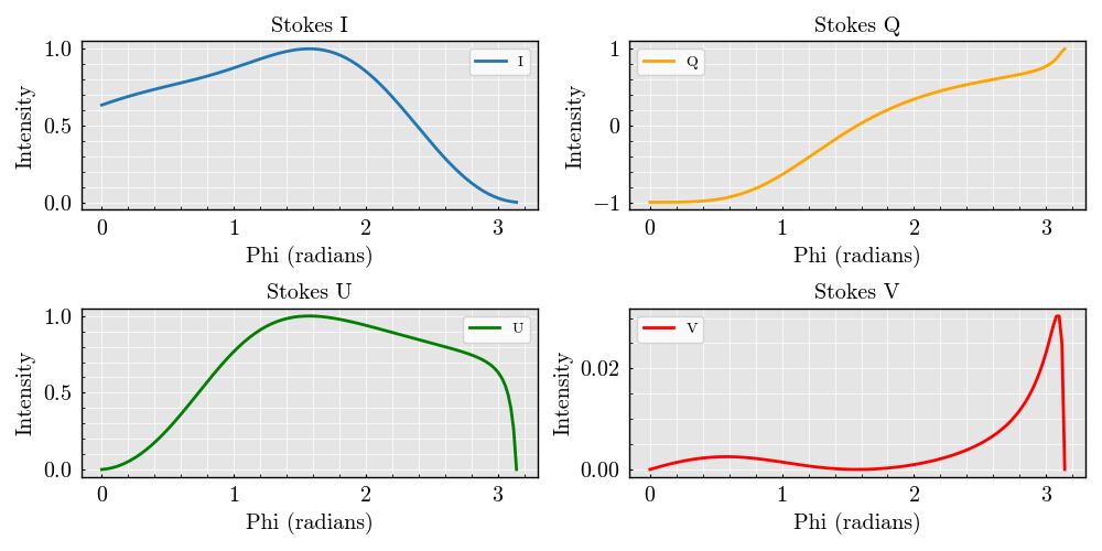
Stokes parameters

I, Q, U, V = scatterer.get_stokes_parameters(phi=phi, theta=theta, distance=1 * ureg.meter )

plt.figure(figsize=(10, 5))
plt.subplot(2, 2, 1)
plt.plot(phi, I, label="I")
plt.title("Stokes I")
plt.xlabel("Phi (radians)")
plt.ylabel("Intensity")
plt.legend()
plt.subplot(2, 2, 2)
plt.plot(phi, Q, label="Q", color="orange")
plt.title("Stokes Q")
plt.xlabel("Phi (radians)")
plt.ylabel("Intensity")
plt.legend()
plt.subplot(2, 2, 3)
plt.plot(phi, U, label="U", color="green")
plt.title("Stokes U")
plt.xlabel("Phi (radians)")
plt.ylabel("Intensity")
plt.legend()
plt.subplot(2, 2, 4)
plt.plot(phi, V, label="V", color="red")
plt.title("Stokes V")
plt.xlabel("Phi (radians)")
plt.ylabel("Intensity")
plt.legend()
plt.tight_layout()
plt.show()